Illuminating the Illuminated – Part Three: Topics of Invention | Topic Modelling the Voynich Manuscript

Srange Tales 016 (Reprint) 015

Our earlier experiments derived some of the darker statistics of the Voynich Manuscript supporting the conjecture, but not erasing all doubt, that the manuscript’s cryptic graphemes are drawn from some natural, or shudderingly unnatural, language.

Despite our beliefs regarding its authenticity, however, the statistical tools we have employed so far can tell us little about the structure, and almost nothing of the meaning, of the Voynich Manuscript. In this post, whilst shying away from the madness and confusion of attempting to translate MS 408, or of definitively identifying its language, we will delve into the extent to which modern natural language processing techniques can reveal its lesser secrets.

The mechanisms we will apply in this post are drawn from the world of topic modelling, an approach widely used in the processing of human language to identify eerily related documents within a corpus of text.

Topic modelling, in its most widely used form, lies in considering each given document as a nebulous admixture of unseen and unknowable topics. These topics, in effect, are themselves probability distributions of words that are likely to occur together. Each document, therefore, is characterised as a set of probability distributions that generate the observed words. This approach, known as Latent Dirichlet Allocation, dispassionately extracts the hidden structure of documents by deriving these underlying distributions.

For known languages, latent Dirichlet allocation extrudes a set of topics characterised by the high-probability words that they generate. These, in turn, can be subjected to human interpretation to identify the semantic underpinnings behind the topics.

To illustrate, we present a topic model of Margaret A. Murray’s seminal 1921 work “The Witch Cult in Western Europe”. There are many uneasy subtleties in producing such a model, into which we will not plunge at this early stage; at a quick glance, however, we can see that from Murray’s detailed research and interweaved arguments for a modern-day survival of an ancient witch cult in Europe, the algorithm can identify certain prevalent themes. The third topic, for example, appears to conjure terms related to the conflict between the accepted state religion and the ‘heathen’ witch cult. The ninth topic concerns itself with the witches’ marks, supposedly identified on the body of practitioners; while the tenth dwells on the clandestine meetings and sabbaths of the cult.

Topic plot for Murray's "The Witch Cult in Western Europe"
Topic plot for Murray’s “The Witch Cult in Western Europe” | (PDF Version)
Witch Cult Topic Model Code

wcwe_topics.r
[code language=”r”]

library( tidyverse )
library( magrittr )

library( ggthemes )
library( showtext )

library( tidytext )
library( widyr )

library( stm )
library( quanteda )

library(cowplot)

# For reorder_within() for facets: <https://juliasilge.com/blog/reorder-within/>
library( drlib )

# Fonts
font_add( "main_font", "/usr/share/fonts/TTF/weird/alchemy/1651 Alchemy/1651AlchemyNormal.otf")
font_add( "bold_font", "/usr/share/fonts/TTF/weird/alchemy/1651 Alchemy/1651AlchemyNormal.otf")

showtext_auto()

# Read (processed) text of Murray’s "The Witch Cult in Western Europe".
wcwe_raw <-
read_csv( "data/wcwe/wcwe_raw.csv", col_names=FALSE ) %>%
rename( text = X1 ) %>%
rowid_to_column( var = "chapter" )

# Tokenize
# (Remove words of 3 letters or less)
# Stemming and stopword removal apparently not so effective anyway,
# according to Schofield et al.: <www.cs.cornell.edu/~xanda/winlp2017.pdf>
wcwe_words <-
wcwe_raw %>%
unnest_tokens( word, text ) %>%
filter( !word %in% stop_words$word ) %>%
filter( str_length( word ) > 3 )

wcwe_word_counts <-
wcwe_words %>%
count( word, chapter, sort = TRUE )

# Generate the corpus
wcwe_dfm <-
wcwe_words %>%
count( chapter, word, sort=TRUE ) %>%
cast_dfm( chapter, word, n )

# Search for a number of topics and output goodness-of-fit measures.

# N=2 is the number of documents ‘held out’ for the goodness-of-fit measure.
# (The model is trained on the main body, then used to calculated the
# likelihood of the held-out documents.) N=2 is used here to produce
# approximately 10% of the corpus.

if( not( file.exists( "work/wcwe_topic_search_k.rds" ) ) ) {

message( "Seaching low-n topic models…" )

wcwe_k <-
searchK( wcwe_dfm, K=c(3:30), N=2 )

saveRDS( wcwe_k, "work/wcwe_topic_search_k.rds" )

} else {

wcwe_k <-
readRDS( "work/wcwe_topic_search_k.rds" )

}

# Plot semantic coherence against exclusivity for model selection
wcwe_k_plot <-
wcwe_k$results %>%
gather( key="variable", value="value", exclus, semcoh )

wcwe_k_semcoh_exclusive <-
ggplot( wcwe_k_plot, aes( x=K, y=value, group=variable) ) +
geom_line() +
facet_wrap( ~variable, ncol=1, scales="free_y" )

# Based on metrics of the above, calculate a 13-topic model
if( not( file.exists( "work/wcwe_topic_stm-13.rds" ) ) ) {

message( "Calculating 13-topic model…" )

wcwe_topic_model_13 <-
stm( wcwe_dfm, K=13, init.type="Spectral" )

# This takes a long time, so save output
saveRDS( wcwe_topic_model_13, "work/wcwe_topic_stm-13.rds" )

} else {

wcwe_topic_model_13 <- readRDS( "work/wcwe_topic_stm-13.rds" )

}

# Work with the 13-topic model for now
wcwe_topic_model <- wcwe_topic_model_13

### Convert output to a tidy tibble
wcwe_topic_model_tbl <-
tidy(wcwe_topic_model, matrix = "beta" )

wcwe_topics_top <-
wcwe_topic_model_tbl %>%
group_by(topic) %>%
top_n(10, beta) %>%
ungroup() %>%
arrange(topic, -beta)

gp <-
wcwe_topics_top %>%
mutate(term = reorder_within(term, beta, topic)) %>%
ggplot(aes(term, beta, fill = factor(topic))) +
geom_col(show.legend = FALSE, alpha=0.8 ) +
facet_wrap(~ topic, scales = "free") +
scale_x_reordered() +
coord_flip()

# Palette of ink colours obtained from screenshots of Diamine inks.
ink_colours <- c( "#753733", "#b6091d", "#e45025", "#232d1d",
"#224255", "#533f50", "#453437", "#7f2430",
"#254673", "#52120e", "#3d2535", "#25464b",
"#2f2a1c" )

gp <-
gp + scale_fill_manual( values=ink_colours )

topic_plot_13 <-
gp + labs( x="Term", y="Probability in Topic" ) +
theme (
plot.title = element_text( family="bold_font", size=16 ),
plot.subtitle = element_text( family="bold_font", size=12 ),
axis.text.y = element_text( family="bold_font", size=10 )
)

theme_set(theme_cowplot(font_size=4, font_family = "main_font" ) )

wcwe_topic_plot <-
topic_plot_13 +
theme (
axis.title.y = element_text( angle = 90, family="main_font", size=12 ),
axis.text.y = element_text( colour="#3c3f4a", family="main_font", size=10 ),
axis.title.x = element_text( colour="#3c3f4a", family="main_font", size=12 ),
axis.text.x = element_text( colour="#3c3f4a", family="main_font", size=10 ),
axis.line.x = element_line( color = "#3c3f4a" ),
axis.line.y = element_line( color = "#3c3f4a" ),
plot.title = element_blank(),
plot.subtitle = element_blank(),
plot.background = element_rect( fill = "transparent" ),
panel.background = element_rect( fill = "transparent" ), # bg of the panel
panel.grid.major.x = element_blank(),
panel.grid.major.y = element_blank(),
panel.grid.minor.x = element_blank(),
panel.grid.minor.y = element_blank(),
legend.text = element_text( family="bold_font", colour="#3c3f4a", size=10 ),
legend.title = element_blank(),
legend.key.height = unit(1.2, "lines"),
legend.position=c(.85,.5),
strip.background = element_blank(),
strip.text.x = element_text(size = 10, family="main_font")
)

# Cowplot trick for ggtitle
title <-
ggdraw() +
draw_label("\"The Witch Cult in Western Europe\" (Murray, 1921) Topic Model", fontfamily="bold_font", colour = "#3c3f4a", size=20, hjust=0, vjust=1, x=0.02, y=0.88) +
draw_label("http://www.weirddatascience.net | @WeirdDataSci", fontfamily="bold_font", colour = "#3c3f4a", size=12, hjust=0, vjust=1, x=0.02, y=0.40)

data_label <-
ggdraw() +
draw_label("Data: Murray, M. \"The Witch Cult in Western Europe\" (1921) | http://www.gutenberg.org/ebooks/20411", fontfamily="bold_font", colour = "#3c3f4a", size=8, hjust=1, x=0.98 )

tgp <-
plot_grid(title, wcwe_topic_plot, data_label, ncol=1, rel_heights=c(0.1, 1, 0.1))

wcwe_topic_plot <-
ggdraw() +
draw_image("img/parchment.jpg", scale=1.4 ) +
draw_plot(tgp)

ggsave( "output/wcwe_topic_plot_13.pdf", width=16, height=9 )

[/code]

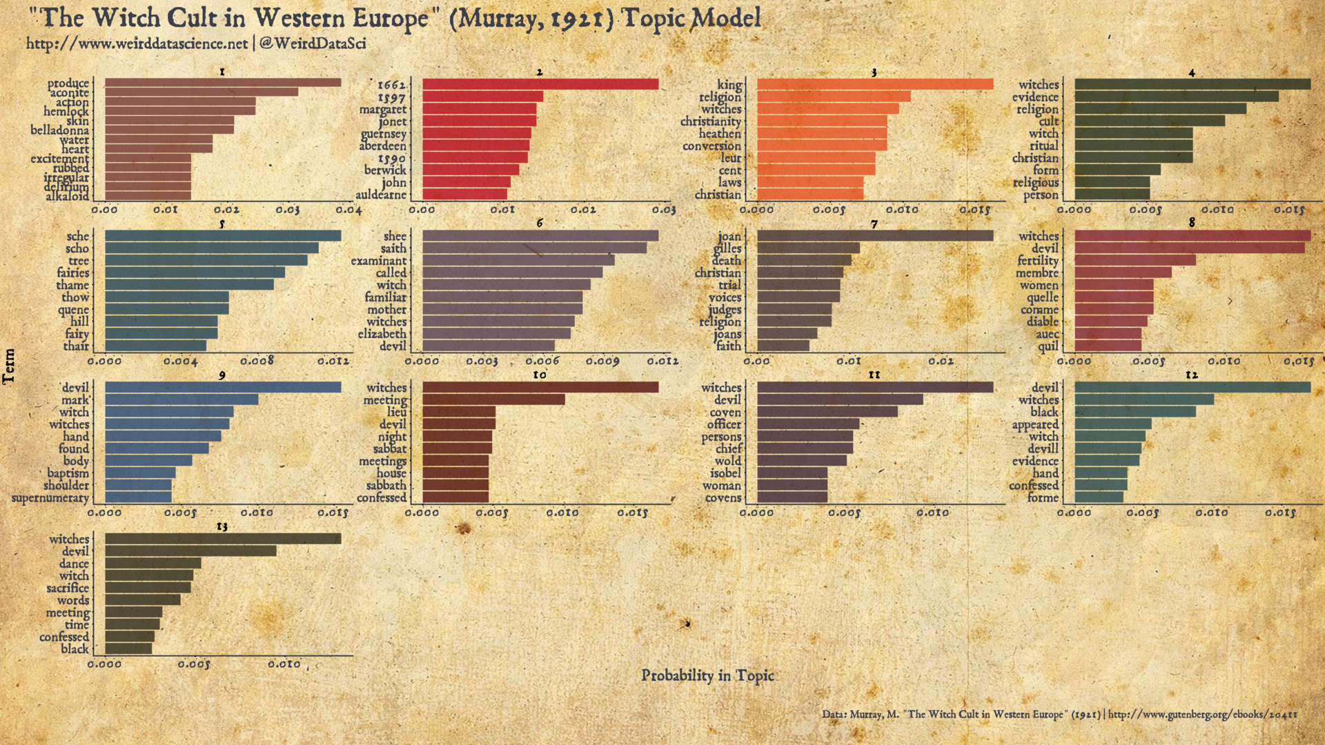
As the plot above suggests, topic modelling is a tool to support our limited human understanding rather than a cold, mechanical source of objectivity and, as with much unsupervised machine learning, there are various subjective choices that must be made guided by the intended purpose of the analysis. Drawing together impercetible threads of relation in bodies of text, the approach suggests major themes and, crucially, can associate disparate areas of text that focus on similar concerns.

Topical Remedies

What, then, can we learn by bringing the oppressive weight of latent Dirichlet allocation to bear against a cryptic tome whose words, and indeed letters, resist our best efforts at interpretation?

Without understanding of individual words, we wil be unable to glean the semantic understanding of topics that was possible with Murray’s Witch Cult…. There is a chance, however, that the topic model can derive relations between separated sections of the manuscript — do certain early pages demonstrate a particular textual relationship to later pages? Do sections of the overall manuscript retain an apparent coherence of topics, with contiguous pages being drawn from a small range of similar topics? Which Voynich words fall under similar topics?

Preparations

Topic modelling typically requires text to undergo a certain level of formulaic preparation. The most common of such rituals are stemming, lemmatization, and stopword removal. Briefly, stemming and lemmatization aim to reduce confusion by rendering words to their purest essence. Stemming is a more crude heuristic, unsympathetically incising endings, and so truncating “dark”, “darker”, “darkest” simply to the atomic root word “dark”. Lemmatization requires more understanding, untangling parts of speech and context: that to curse is a verb while a curse is a noun; the two identical words should therefore be treated separately.

Stopword removal aims to remove the overwhelming proportion of shorter, structural words that are ubiquitous throughout any text, but are largely irrelevant to the overall topic: the, and, were, it, they, but, if…. Whilst key to our understanding of texts, these terms have no significance to the theme or argument of a text.

Undermining our scheme to perform topic modelling, therefore, is the lamentable fact that, without understanding of either the text or its structure, we are largely unable to perform any of these tasks satisfactorily. We have neither an understanding of the grammatical form of Voynich words allowing stemming or lemmatization, or a list of stopwords to excise.

Whilst stemming and lemmatization are unapproachable, at least within the confines of this post, we can effect a crude form of stopword removal through use of a common frequency analysis of the text. Stopwords are, in general, those words that are both most-frequently occuring in some corpus of documents and those that are found across the majority of documents in that language. The second criterion ensures that words occurring frequently in obscure and specialised texts are not considered of undue importance.

This overall statistic is known as term frequency-inverse document frequency, or tf-idf, and is widely used in information retrieval to identify terms of specific interest within certain documents that are not shared by the wider corpus. For our purposes, we wish to identify and elide those ubiquitous, frequent terms that occur across the entire corpus. To do so, given our lack of knowledge of the structure of the Voynich Manuscript, we will consider each folio as a separate document, and consider only the inverse document frequency as we are uninterested in how common a word within each document. To avoid words that most commonly appear across the manuscript, with a basis in the distribution of stop words in a range of known languages, we therefore remove the 200 words with lowest inverse document frequency scores1.

Having contorted the text into an appropriate form for analysis, we can begin the process of discerning its inner secrets. Our code relies on the tidytext and stm packages, allowing for easy manipulation of document structure and topic models2

Numerous Interpretations

Topic models are a cautionary example of recklessly unsupervised machine learning. As with most such approaches, there are a number of subjective choices to be made that affect the outcome. Perhaps the most influential is the selection of the number of topics that the model should generate. Whilst some approaches have been suggested to derive this number purely by analysis, in most cases it remains in the domain of the human supplicant. Typically, the number of topics is guided both by the structure of the text along with whatever arcane purpose the analysis might have. With our imposed lack of understanding, however, we must rely solely on crude metrics to make this most crucial of choices.

Several methods of assessment exist to quantify the fit of a topic model to the text. The two that we will employ, guided by the stm package are semantic coherence, which roughly expresses that words from a given topic should co-occur within a document; and exclusivity, which values models more highly when given words occur within topics with high frequency, but are also relatively exclusive to those topics.

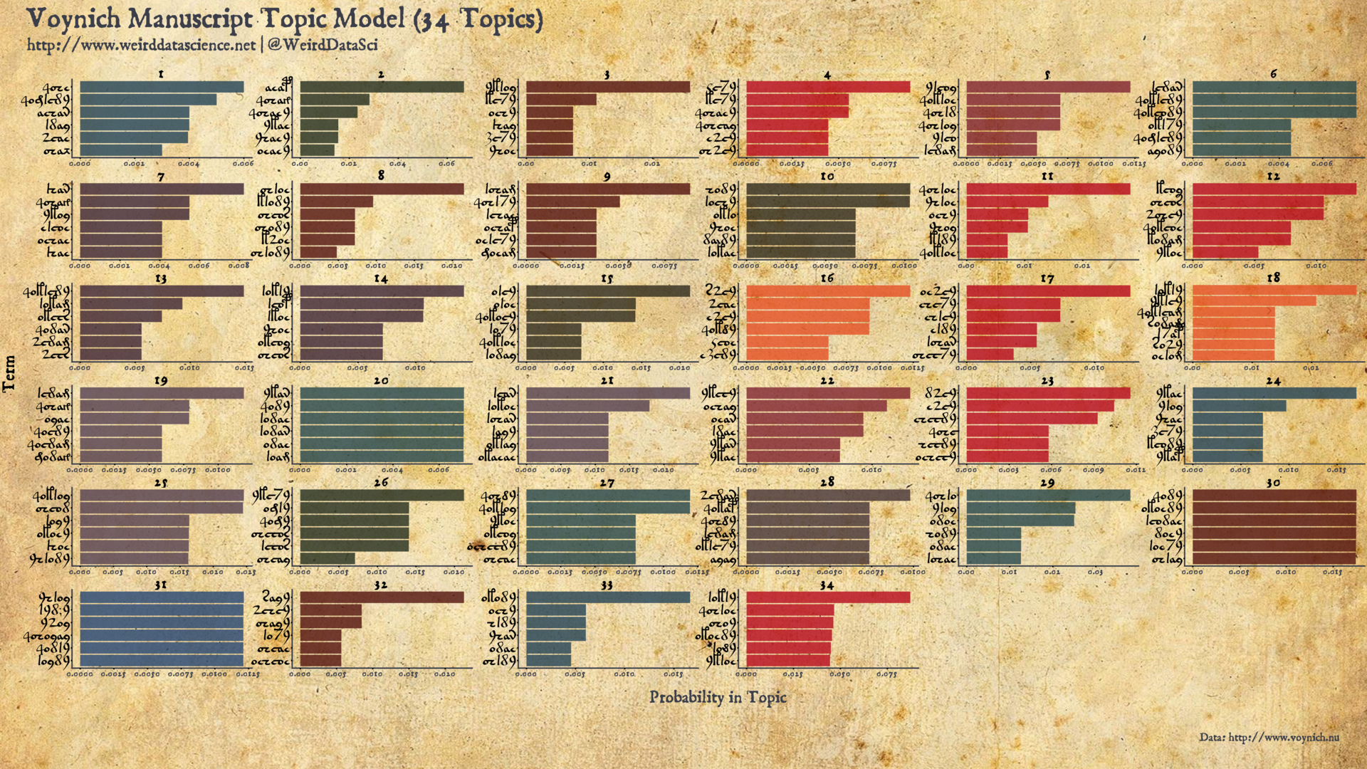
We select an optimal number of topics by the simple process of calculating models with varying numbers of topics, and assessing when these two scores are maximised. For the Voynich Manuscript we observe that 34 topics appears to be initially optimal3.

Voynich Topic Model Selection Metrics
Selection metrics for Voynich topic model topic numbers. | (PDF Version)

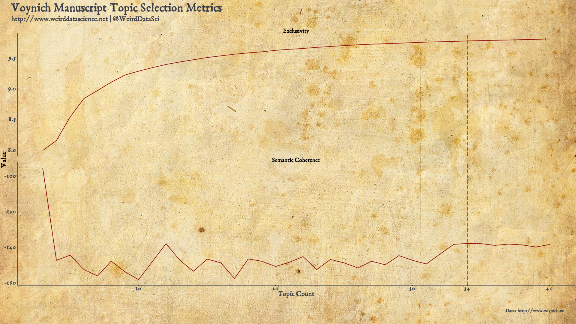
The initial preparation of the code, the search through topic models of varying numbers, and the selection of the final 34 topic model is given in the code below alongside plotting code for the metrics diagram.

Voynich Manuscript Topic Modelling Code

voynich_topics-model.r
[code language=”r”]

library( tidyverse )
library( magrittr )

library( tidytext )
library( widyr )

library( stm )

# install_github("dgrtwo/drlib")
library( drlib )

# References:
# <http://varianceexplained.org/r/op-ed-text-analysis/>
# <https://cbail.github.io/SICSS_Topic_Modeling.html#working-with-meta-data>
# <https://me.eui.eu/andrea-de-angelis/blog/structural-topic-models-to-study-political-text-an-application-to-the-five-star-movements-blog/>
# <https://scholar.princeton.edu/sites/default/files/bstewart/files/stm.pdf>
# <https://juliasilge.com/blog/evaluating-stm/>

voynich_raw <-
read_csv( "data/voynich_raw.txt", col_names=FALSE ) %>%
rename( folio = X1, text = X2 )

# Read in manually-identiied sections per folio, according to
# <http://www.voynich.nu/descr.html#illustr>
voynich_sections <-
read_csv( "data/voynich_sections.txt", col_names=FALSE ) %>%
rename( folio = X1, section = X2 )

# Merge the above to note section for each folio alongside the text
voynich_tbl <-
left_join( voynich_sections, voynich_raw )

# Tokenize
# Remove words of 3 letters or less.
voynich_words <-
voynich_tbl %>%
unnest_tokens( word, text ) %>%
filter( str_length( word ) > 3 )

# Most common words
voynich_common <-
voynich_words %>%
count( word, sort=TRUE ) %>%
mutate( word = reorder( word, n ) )

# Counts of words per folio
voynich_word_counts <-
voynich_words %>%
count( word, folio, sort = TRUE )

# TF-IDF
voynich_tf_idf <-
voynich_word_counts %>%
bind_tf_idf( word, folio, n ) %>%
arrange( desc( tf_idf ) )

# Based on median stopword count of languages in NLTK
# (<https://raw.githubusercontent.com/nltk/nltk_data/gh-pages/packages/corpora/stopwords.zip>),
# remove the 200 lowest-scoring words.
voynich_stopwords <-
voynich_tf_idf %>%
arrange( idf ) %>%
select( word ) %>%
unique() %>%
head( 200 ) %>%
extract2( "word" )

voynich_words <-
voynich_words %>%
filter( !word %in% voynich_stopwords )

# Generate the corpus
voynich_dfm <-
voynich_words %>%
count( folio, word, sort=TRUE ) %>%
cast_dfm( folio, word, n )

# Search for a number of topics and output goodness-of-fit measures.

# N=20 is the number of documents ‘held out’ for the goodness-of-fit measure.
# (The model is trained on the main body, then used to calculated the
# likelihood of the held-out documents.) N=20 is used here to produce
# approximately 10% of the corpus.
if( not( file.exists( "work/voynich_topic_search_k.rds" ) ) ) {

message( "Seaching low-n topic models…" )

voynich_k <-
searchK( voynich_dfm, K=c(3:40), N=20 )

saveRDS( voynich_k, "work/voynich_topic_search_k.rds" )

} else {

voynich_k <-
readRDS( "work/voynich_topic_search_k.rds" )

}

# Based on the metrics above, use 34-topic model
if( not( file.exists( "work/voynich_topic_stm-34.rds" ) ) ) {

message( "Calculating 34-topic model…" )

# Setting K=0 uses (Lee and Minno, 2014) to select a number of topics
voynich_topic_model_34 <-
stm( voynich_dfm, K=34, init.type="Spectral" )

# This takes a long time, so save output
saveRDS( voynich_topic_model_34, "work/voynich_topic_stm-34.rds" )

} else {

voynich_topic_model_34 <- readRDS( "work/voynich_topic_stm-34.rds" )

}

# Based on the metrics above, also calculated a secondary 12-topic model
if( not( file.exists( "work/voynich_topic_stm-12.rds" ) ) ) {

message( "Calculating 12-topic model…" )

# Setting K=0 uses (Lee and Minno, 2014) to select a number of topics
voynich_topic_model_12 <-
stm( voynich_dfm, K=12, init.type="Spectral" )

# This takes a long time, so save output
saveRDS( voynich_topic_model_12, "work/voynich_topic_stm-12.rds" )

} else {

voynich_topic_model_12 <- readRDS( "work/voynich_topic_stm-12.rds" )

}

# Work initially with the 34-topic model
voynich_topic_model <- voynich_topic_model_34

## Convert output to a tidy tibble
voynich_topic_model_tbl <-
tidy(voynich_topic_model, matrix = "beta" )

voynich_terms <-
tidy(voynich_topic_model, matrix = "gamma" )

# Select the top six terms in each topic for display
voynich_topics_top <-
voynich_topic_model_tbl %>%
group_by(topic) %>%
top_n(6, beta) %>%
ungroup() %>%
arrange(topic, -beta)

# Produce a per-folio topic identification.
# Document – topic – score
topic_identity <-
voynich_terms %>%
group_by( document ) %>%
top_n( 1, gamma ) %>%
arrange( document ) %>%
ungroup

# Reinsert manually-identified section information (derived from
# illustrations).
topic_identity$section <- voynich_tbl$section

saveRDS( topic_identity, "work/topic_identity.rds" )

[/code]
Topic Metric Selection Plotting Code

voynich_topics-plot_metric.r
[code language=”r”]

library( tidyverse )
library( magrittr )

library( ggthemes )
library( showtext )

library( ggplot2 )
library( cowplot )

# References:
# <http://varianceexplained.org/r/op-ed-text-analysis/>
# <https://cbail.github.io/SICSS_Topic_Modeling.html#working-with-meta-data>
# <https://me.eui.eu/andrea-de-angelis/blog/structural-topic-models-to-study-political-text-an-application-to-the-five-star-movements-blog/>
# <https://scholar.princeton.edu/sites/default/files/bstewart/files/stm.pdf>
# <https://juliasilge.com/blog/evaluating-stm/>

font_add( "voynich_font", "/usr/share/fonts/TTF/weird/voynich/eva1.ttf")
font_add( "main_font", "/usr/share/fonts/TTF/weird/alchemy/1651 Alchemy/1651AlchemyNormal.otf")
font_add( "bold_font", "/usr/share/fonts/TTF/weird/alchemy/1651 Alchemy/1651AlchemyNormal.otf")

showtext_auto()

# Read topic model search
voynich_k <-
readRDS( "work/voynich_topic_search_k.rds" )

# Plot semantic coherence against exclusivity for model selection
voynich_k_plot <-
voynich_k$results %>%
as_tibble %>%
rename( "Semantic Coherence"=semcoh, "Exclusivity"=exclus ) %>%
gather( key="variable", value="value", "Semantic Coherence", "Exclusivity" ) %>%
rename( "Topic Count"=K, "Value"=value )

# We will use cowplot, so set the theme here.
theme_set(theme_cowplot(font_size=4, font_family = "main_font" ) )

# Plot semantic coherence against exclusivity.
# (Highlight the selected 34-topic point.)
voynich_k_semcoh_exclusive <-
ggplot( voynich_k_plot, aes( x=`Topic Count`, y=Value, group=variable) ) +
geom_line( colour="#8a0707" ) +
facet_wrap( ~variable, ncol=1, scales="free_y" ) +
geom_vline( xintercept=34, colour="#228b22", linetype="longdash" ) +
scale_x_continuous(breaks=c( seq(0, 40, 10), 34 ) ) +
theme (
axis.title.y = element_text( angle = 90, family="main_font", size=12 ),
axis.title.x = element_text( colour="#3c3f4a", family="main_font", size=12 ),
axis.text.x = element_text( colour="#3c3f4a", family="main_font", size=10 ),
axis.text.y = element_text( colour="#3c3f4a", family="main_font", size=10 ),
axis.line.x = element_line( color = "#3c3f4a" ),
axis.line.y = element_line( color = "#3c3f4a" ),
plot.title = element_blank(),
plot.subtitle = element_blank(),
plot.background = element_rect( fill = "transparent" ),
panel.background = element_rect( fill = "transparent" ), # bg of the panel
panel.grid.major.x = element_blank(),
panel.grid.major.y = element_blank(),
panel.grid.minor.x = element_blank(),
panel.grid.minor.y = element_blank(),
legend.text = element_text( family="bold_font", colour="#3c3f4a", size=10 ),
legend.title = element_blank(),
legend.key.height = unit(1.2, "lines"),
legend.position=c(.85,.5),
strip.background = element_blank(),
strip.text.x = element_text(size = 10, family="main_font")
)

# Cowplot trick for ggtitle
title <-
ggdraw() +
draw_label("Vonich Manuscript Topic Selection Metrics", fontfamily="bold_font", colour = "#3c3f4a", size=20, hjust=0, vjust=1, x=0.02, y=0.88) +
draw_label("http://www.weirddatascience.net | @WeirdDataSci", fontfamily="bold_font", colour = "#3c3f4a", size=12, hjust=0, vjust=1, x=0.02, y=0.40)

data_label <-
ggdraw() +
draw_label("Data: http://www.voynich.nu", fontfamily="bold_font", colour = "#3c3f4a", size=8, hjust=1, x=0.98 )

tgp <-
plot_grid(title, voynich_k_semcoh_exclusive, data_label, ncol=1, rel_heights=c(0.1, 1, 0.1))

voynich_topic_selection_plot <-
ggdraw() +
draw_image("img/parchment.jpg", scale=1.4 ) +
draw_plot(tgp)

ggsave( "output/voynich_topic_selection_metrics.pdf", width=16, height=9 )

[/code]

With these torturous steps on our path finally trodden, our path leads at last to a model deriving the underlying word generating probabilities of the Voynich Manuscript. In each facet, the highest-probability words in each topic are shown in order.

Voynich Manuscript Topic Model
Voynich Manuscript Topic Model (34 topics) | (PDF Version)
Topic Model Plotting Code

voynich_topics-plot_topics.r
[code language=”r”]

library( tidyverse )
library( magrittr )

library( ggthemes )
library( showtext )

library( tidytext )

# install_github("dgrtwo/drlib")
library( drlib )

library( ggplot2 )
library( cowplot )

font_add( "voynich_font", "/usr/share/fonts/TTF/weird/voynich/eva1.ttf")
font_add( "main_font", "/usr/share/fonts/TTF/weird/alchemy/1651 Alchemy/1651AlchemyNormal.otf")
font_add( "bold_font", "/usr/share/fonts/TTF/weird/alchemy/1651 Alchemy/1651AlchemyNormal.otf")

showtext_auto()

# ####################
# ## 34 Topic Model ##
# ####################

# Work with the 34-topic model
voynich_topic_model <-
readRDS( "work/voynich_topic_stm-34.rds" )

## Convert output to a tidy tibble
voynich_topic_model_tbl <-
tidy(voynich_topic_model, matrix = "beta" )

voynich_terms <-
tidy(voynich_topic_model, matrix = "gamma" )

# Select the top six terms in each topic for display
voynich_topics_top <-
voynich_topic_model_tbl %>%
group_by(topic) %>%
top_n(6, beta) %>%
ungroup() %>%
arrange(topic, -beta)

# We will use cowplot, so set the theme here.
theme_set(theme_cowplot(font_size=4, font_family = "main_font" ) )

# Plot each topic as a geom_col(). Use drlib’s ‘reorder_within’ to order bars
# within each facet. (Note that the scale_x_reordered() is needed to fix
# (flipped!) x-axis labels in the output.)
# <https://juliasilge.com/blog/reorder-within/>
gp <-
voynich_topics_top %>%
mutate(term = reorder_within(term, beta, topic)) %>%
ggplot(aes(term, beta, fill = factor(topic))) +
geom_col( alpha=0.8, show.legend = FALSE) +
theme( axis.text.y = element_text( family="voynich_font", size=10 ) ) +
facet_wrap(~ topic, scales = "free") +
scale_x_reordered() +
coord_flip() +
labs( x="Term", y="Probability in Topic" )

# Theming
gp <-
gp +
theme (
axis.title.y = element_text( margin = margin(t = 0, r = 12, b = 0, l = 0), angle = 90, family="main_font", size=12 ),
axis.title.x = element_text( margin = margin(t = 12, r = 0, b = 0, l = 0), colour="#3c3f4a", family="main_font", size=12 ),
axis.text.x = element_text( colour="#3c3f4a", family="main_font", size=6 ),
axis.line.x = element_line( color = "#3c3f4a" ),
axis.line.y = element_line( color = "#3c3f4a" ),
plot.title = element_blank(),
plot.subtitle = element_blank(),
plot.background = element_rect( fill = "transparent" ),
panel.background = element_rect( fill = "transparent" ), # bg of the panel
panel.grid.major.x = element_blank(),
panel.grid.major.y = element_blank(),
panel.grid.minor.x = element_blank(),
panel.grid.minor.y = element_blank(),
legend.text = element_text( family="bold_font", colour="#3c3f4a", size=10 ),
legend.title = element_blank(),
legend.key.height = unit(1.2, "lines"),
legend.position=c(.85,.5),
strip.background = element_blank(),
strip.text.x = element_text(size = 10, family="main_font")
)

gp <-
gp +
theme(
panel.background = element_rect(fill = "transparent", colour = "transparent"),
plot.background = element_rect(fill = "transparent", colour = "transparent"),
legend.background = element_rect(fill = "transparent", colour = "transparent")
)

# Palette of ink colours (based on screenshots of Diamine inks).
ink_colours <- c( "#753733", "#b6091d", "#e45025", "#232d1d",
"#224255", "#533f50", "#453437", "#7f2430",
"#254673", "#52120e", "#3d2535", "#25464b",
"#2f2a1c" )

# Create a vector of selections from the palette, one for each topic.
ink_palette <-
sample( ink_colours, size=34, replace=TRUE )

# Add fill colours to plot.
gp <-
gp + scale_fill_manual( values=ink_palette )

# Cowplot trick for ggtitle
title <-
ggdraw() +
draw_label("Vonich Manuscript Topic Model (34 Topics)", fontfamily="bold_font", colour = "#3c3f4a", size=20, hjust=0, vjust=1, x=0.02, y=0.88) +
draw_label("http://www.weirddatascience.net | @WeirdDataSci", fontfamily="bold_font", colour = "#3c3f4a", size=12, hjust=0, vjust=1, x=0.02, y=0.40)

data_label <-
ggdraw() +
draw_label("Data: http://www.voynich.nu", fontfamily="bold_font", colour = "#3c3f4a", size=8, hjust=1, x=0.98 )

tgp <-
plot_grid(title, gp, data_label, ncol=1, rel_heights=c(0.1, 1, 0.1))

voynich_topic_plot <-
ggdraw() +
draw_image("img/parchment.jpg", scale=1.4 ) +
draw_plot(tgp)

ggsave( "output/voynich_topic_plot_34.pdf", width=16, height=9 )

[/code]

Of Man and Machine

The topic model produces a set of topics in the form of probability distributions generating words. The association of each topic to a folio in the Voynich Manuscript represents these probabilistic assignments based solely on the distribution of words in the text. There is a secondary topic identification, however, tentatively proposed by scholars of the manuscript. The obscure diagrams decorating almost every folio provide their own startling implications as to the themes detailed in the undeciphered prose.

We might wish to ask, then: do the topic assignments generated by the machine reflect the human intepretation? To what extent do pages decorated with herbal illuminations follow certain machine-identified topics compared with those assigned to astronomical charts?

The illustration-based thematic sections of the Voynich Manuscript fall into eight broad categories, according to Zandbergen. These sections are, briefly:

  • Herbal, detailing a range of unidentified plants, comprising most of the first half of the manuscript;
  • astronomical, focusing on stars, planets, and astronomical symbols;
  • cosmological, displaying obscure circular diagrams of a similar form to the astronomical;
  • astrological, in which small humans are displayed mostly in circular diagrams alongside zodiac signs;
  • biological, characterised by small drawings of human figures, often connected by tubes;
  • pharmaceutical, detailing parts of plants and vessels for their preparation;
  • starred text, divided into short paragraphs marked with a star, with no other illustrations; and
  • text only pages.

With these contextual descriptions, we can examine the relationship between the speculative assignments of the topic model against the suggestions of the diagrams.

Voynich Manuscript Folio Topic Heatmap
Voynich Manuscript Folio Topic Heatmap | (PDF Version)
Voynich Manuscript Topic Model Folio Heatmap Plotting Code

voynich_topics-plot_heatmap.r
[code language=”r”]

library( tidyverse )
library( magrittr )

library( ggthemes )
library( showtext )

# install_github("dgrtwo/drlib")
library( drlib )

library( ggplot2 )
library( cowplot )

font_add( "main_font", "/usr/share/fonts/TTF/weird/alchemy/1651 Alchemy/1651AlchemyNormal.otf")
font_add( "bold_font", "/usr/share/fonts/TTF/weird/alchemy/1651 Alchemy/1651AlchemyNormal.otf")

showtext_auto()

# Set the number of topics
n_topics <- 34

# Load the appropriate topic model
voynich_topic_model <-
readRDS( paste0( "work/voynich_topic_stm-", n_topics, ".rds" ))

theme_set(theme_cowplot(font_size=4, font_family = "main_font" ) )

# Load folio topic identity assignments
topic_identity <-
readRDS( "work/topic_identity.rds" )

# Cowplot
theme_set(theme_cowplot(font_size=4, font_family = "main_font" ) )

# Plot topic heatmap
topic_heatmap <-
topic_identity %>%
ggplot( aes( x=document, y=topic, fill=section ) ) +
geom_tile( colour="#3c3f4a", alpha=0.8, size=0.4 ) +
scale_fill_brewer( palette="Dark2", direction=1, name="Section", labels=c("Astrological", "Astronomical", "Biological", "Cosmological", "Herbal", "Pharmaceutical", "Starred Text", "Text Only" ) ) +
ggtitle( "Voynich Folio Topic Assignments", paste( n_topics, "Topic Model" )) +
labs( x="Folio", y="Topic" ) +
theme (
plot.title = element_text( family="bold_font", size=22 ),
plot.subtitle = element_text( family="bold_font", size=12 ),
panel.grid.major.x = element_blank(),
panel.grid.major.y = element_blank(),
panel.grid.minor.x = element_blank(),
panel.grid.minor.y = element_blank(),
) +
scale_y_continuous(labels = seq( 1, n_topics, 1 ), breaks = seq( 1, n_topics, 1 ), minor_breaks = seq(0.5 , n_topics+.5, 1) ) +
scale_x_continuous(minor_breaks = seq(0.5 , 226.5, 5) )

gp <-
topic_heatmap +
theme (
axis.title.y = element_text( margin = margin(t = 0, r = 12, b = 0, l = 0), angle = 90, family="main_font", size=12 ),
axis.title.x = element_text( colour="#3c3f4a", family="main_font", size=12 ),
axis.text.x = element_text( colour="#3c3f4a", family="main_font", size=10 ),
axis.text.y = element_text( colour="#3c3f4a", family="main_font", size=10 ),
axis.line.x = element_line( color = "#3c3f4a" ),
axis.line.y = element_line( color = "#3c3f4a" ),
plot.title = element_blank(),
plot.subtitle = element_blank(),
plot.background = element_rect( fill = "transparent" ),
panel.background = element_rect( fill = "transparent" ), # bg of the panel
legend.text = element_text( family="bold_font", colour="#3c3f4a", size=10 ),
legend.title =element_text( family="bold_font", colour="#3c3f4a", size=12 ),
legend.key.height = unit(1.2, "lines"),
strip.background = element_blank(),
strip.text.x = element_text(size = 10, family="main_font")
)

gp <-
gp +
theme(
panel.background = element_rect(fill = "transparent", colour = "transparent"),
plot.background = element_rect(fill = "transparent", colour = "transparent"),
legend.background = element_rect(fill = "transparent", colour = "transparent")
)

# Cowplot trick for ggtitle
title <-
ggdraw() +
draw_label("Voynich Manuscript Topic Heatmap", fontfamily="bold_font", colour = "#3c3f4a", size=20, hjust=0, vjust=1, x=0.02, y=0.88) +
draw_label("http://www.weirddatascience.net | @WeirdDataSci", fontfamily="bold_font", colour = "#3c3f4a", size=12, hjust=0, vjust=1, x=0.02, y=0.40)

data_label <-
ggdraw() +
draw_label("Data: http://www.voynich.nu", fontfamily="bold_font", colour = "#3c3f4a", size=8, hjust=1, x=0.98 )

tgp <-
plot_grid(title, gp, data_label, ncol=1, rel_heights=c(0.1, 1, 0.1))

voynich_topic_heatmap <-
ggdraw() +
draw_image("img/parchment.jpg", scale=1.4 ) +
draw_plot(tgp)

ggsave( "output/voynich_folio_topic_heatmap.pdf", width=16, height=9 )

[/code]

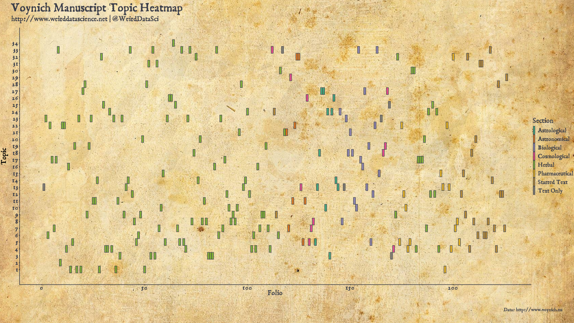
The colours in the above plot represent the manual human interpretation, whilst the location on the y-axis shows the latent Dirichlet allocation topic assignment.

We might have harboured the fragile hope that such a diagram would have demonstrated a clear confirmatory delineation between the sectional diagrammatic breakdown of the Voynich Manuscript. At a first inspection, however, the topics identified by the analysis appear almost uniformly distributed across the pages of the manuscript.

The topic model admits to a number of assumptions, not least the selection of stopwords through to the number of topics in the model. We must also be cautious: the apparent distribution of topics over the various sections may be deceptive. For the moment, we can present this initial topic model as a faltering first step in our descent into the hidden structures of the Voynich Manuscript. The next, and final, post in this series will develop both the statistical features and the topic model towards a firmer understanding of whether the apparent shift in theme suggest by the illustrations is statistically supported by the text.

Until then, read deeply but do not trust what you read.


Footnotes

  1. The widely-used NLTK stopword corpus contains a list of stopwords for 23 world languages, with a notable bias towards European languages. The median length of these stopword lists is 201.5, with values ranging from 53 for Turkish to 1784 for Slovene.
  2. We have also relied extensively on the superb work and writing of Silge on this topic.
  3. It should be noted that topic modelling is more typically applied to much larger corpora of text than is possible with our restriction to the Voynich Manuscript. Given the relatively short nature of the text, we might prefer to focus on a smaller number of topics. The metrics plot shows a spike in semantic coherence around 12 topics that might be of interest in future analyses.

Be the first to comment

Leave a Reply

Your email address will not be published.


This site uses User Verification plugin to reduce spam. See how your comment data is processed.

This site uses Akismet to reduce spam. Learn how your comment data is processed.