In the previous post in this series we coyly unveiled the tantalising mysteries of the Voynich Manuscript: an early 15th century text written in an unknown alphabet, filled with compelling illustrations of plants, humans, astronomical charts, and less easily-identifiable entities.
Stretching back into the murky history of the Voynich Manuscript, however, is the lurking suspicion that it is a fraud; either a modern fabrication or, perhaps, a hoax by a contemporary scribe.
One of the more well-known arguments for the authenticity of the manuscript, in addition to its manufacture with period parchment and inks, is that the text appears to follow certain statistical properties associated with human language, and which were unknown at the time of its creation.
The most well-known of these properties is that the frequency of words in the Voynich Manuscript have been claimed to follow a phenomenon known as Zipf’s Law, whereby the frequency of a word’s occurrence in the text is inversely proportional to its rank in the list of words ordered by frequency.
In this post, we will scrutinise the extent to which the expected statistical properties of natural languages hold for the arcane glyphs presented by the Voynich manuscript.
Unnatural Laws
Zipf’s Law is an example of a discrete power law probability distribution. Power laws have been found to lurk beneath a sinister variety of ostensibly natural phenomena, from the relative size of human settlements to the diversity of species descended from a particular ancestral freshwater fish.
In its original context of human langauge, Zipf’s Law states that the most common word in a given language is likely to be roughly twice as common as the second most common word, and three times as common as the third most common word. More precisely, this law holds for much of the corpus, as the law tends to break down somewhat at both the most-frequent and least-frequent words in the corpus1. Despite this, we will focus on the original, simpler Zipfian characterisation in this analysis.
More generally, it is rarely sensible to claim that any natural phenomenon follows a given distribution or model, but instead to demonstrate that a distribution presents a useful model for a given set of observations. Indeed, it is possible to fit any set of observations to a power law, with the assumption that the fit will be poor. Ultimately, we can do little more than demonstrate that a given model is the best simulacrum of observed reality, subject to the uses to which it will be put. Certainly, a more Bayesian approach would advocate building a range of models, demonstrating that the power law is most accurate. All truth, it seems, is relative.
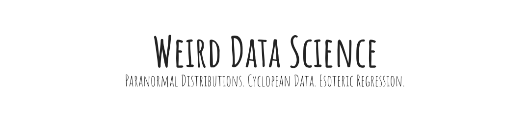
Faced with the awful statistical horror of the universe, we are reduced to seeking evidence against a phenomenon’s adherence to a given distribution. Our first examination, then, is to see whether the basic log-log plot supports or undermines the Voynich Manuscript.
Fitted Power Law of Voynich Corpus | (PDF Version)
A crude visual analysis certainly supports the argument that, for much of the upper half of the Voynich corpus, there is a linear relationship on the log-log plot consistent with Zipf’s Law. As mentioned, however, this superficial appeal to our senses leaves a gnawing lack of certainty in the conclusion. We must turn to less fallible tools.
The poweRlaw package for R is designed specifically to exorcise these particular demons. This package attempts to fit a power law distribution to a series of observations, in our case the word frequencies observed in the corpus of Voynich text. With the fitted model, we then attempt to disprove the null hypothesis that the data is drawn from a power law. If this attempt to betray our own model fails, then we attain an inverse enlightenment: there is insufficient evidence that the model is not drawn from a power law.
This is an inversion of the more typical frequentist null hypothesis scenario. Typically, in such approaches, we hope for a low p-value, typically below 0.05 or even 0.001, showing that the chance of the observations being consistent with the null hypothesis is extremely low. For this test, we instead hope that our p-value is insufficiently low to make such a claim, and thus that a power law is consistent with the data.
The diagram above shows a fitted parameterisation of the power law according to the poweRlaw package. In addition to the visually appealing fit of the line, the weirdly inverted logic of the above test provides a p-value of 0.151. We thus have as much confidence as we can have, via this approach, that a power law is a reasonable model for the text in the Voynich corpus.
# Tokenize
voynich_words <-
voynich_tbl %>%
unnest_tokens( word, text )
# Most common words
message( "Calculating Voynich language statistics…" )
voynich_common <-
voynich_words %>%
count( word, sort=TRUE ) %>%
mutate( word = reorder( word, n ) ) %>%
mutate( freq = n / sum(n) )
# (Following the poweRlaw vignette)
# Create a discrete power law distribution object from the word counts
voynich_powerlaw <-
voynich_common %>%
extract2( "n" ) %>%
displ$new()
# Estimate the lower bound
voynich_powerlaw_xmin <-
estimate_xmin( voynich_powerlaw )
# Set the parameters of the voynich_powerlaw to the estimated values
voynich_powerlaw$setXmin( voynich_powerlaw_xmin )
# Estimate parameters of the power law distribution
voynich_powerlaw_est <-
estimate_pars( voynich_powerlaw )
# Calculate p-value of power law. See Section 4.2 of "Power-Law Distributions in Empirical Data" by Clauset et al.
# If the p-value is _greater_ than 0.1 then we cannot rule out a power-law distribution.
voynich_powerlaw_bootstrap_p <-
bootstrap_p(voynich_powerlaw, no_of_sims=1000, threads=7 )
# p=0.143 power law cannot be ruled out
# Plot data and power law fit
voynich_powerlaw_plot_data <-
plot( voynich_powerlaw, draw = F ) %>%
mutate(
log_x = log( x ),
log_y = log( y ) )
voynich_powerlaw_fit_data <-
lines( voynich_powerlaw, col=2, draw = F ) %>%
mutate(
log_x = log( x ),
log_y = log( y )
)
# Plot the fitted power law data.
gp <-
ggplot( voynich_powerlaw_plot_data ) +
geom_point( aes( x = log( x ), y =log( y ) ), colour="#8a0707" ) +
geom_line( data= voynich_powerlaw_fit_data,
aes(
x = log( x ),
y = log( y ) ), colour="#0b6788") +
labs(
x = "Log Rank",
y = "Log Frequency" )
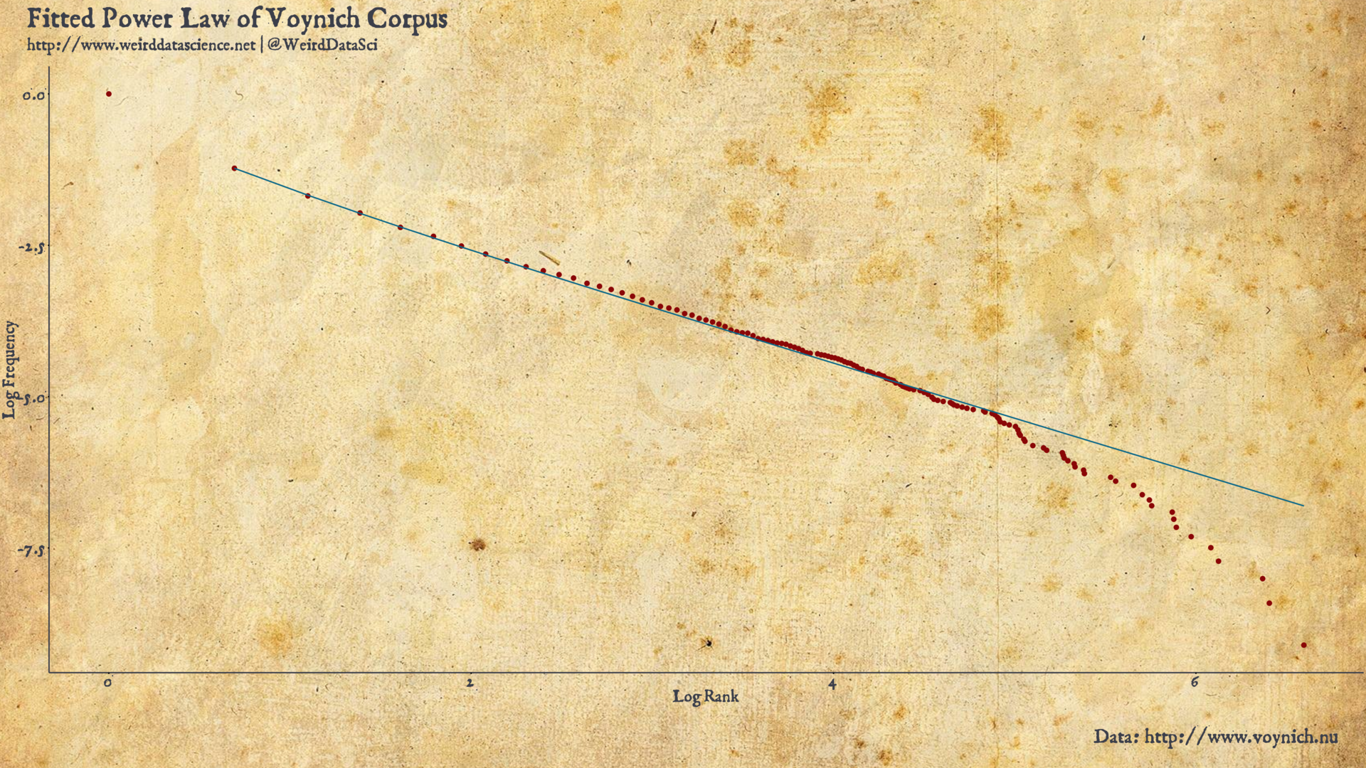
Led further down twisting paths by this initial taste of success, we can now present the Voynich corpus against other human-language corpora to gain a faint impression of how similar or different it is to known languages. The following plot compares the frequency of words in the Voynich Manuscript to those of the twenty most popular languages in Wikipedia, taken from the dataset available here.
Voynich Manuscript Rank Frequency Distribution against Wikipedia Corpora | (PDF Version)
# Tokenize
# (Remove words of 3 letters or less)
# Stemming and stopword removal apparently not so effective anyway,
# according to Schofield et al.: <www.cs.cornell.edu/~xanda/winlp2017.pdf>
voynich_words <-
voynich_tbl %>%
unnest_tokens( word, text )
# Most common words
message( "Calculating Voynich language statistics…" )
voynich_common <-
voynich_words %>%
count( word, sort=TRUE ) %>%
mutate( word = reorder( word, n ) ) %>%
mutate( freq = n / sum(n) )
# Plot a log-log plot of Voynich word frequencies.
voynich_word_counts <-
voynich_words %>%
count( word, folio, sort = TRUE )
# Load other languages.
# Select frequency counts.
# Convert to long format, then normalise per-language.
message( "Loading common language statistics…" )
wiki_language <-
read.csv( "data/Multilingual_Wikipedia_2015_word_frequencies__32_languages_X_5_million_words.csv" ) %>%
head( 10000 ) %>%
as_tibble %>%
select( matches( "*_FREQ" ) ) %>%
gather( key = "language", value = "count" ) %>%
mutate( language = str_replace( language, "_FREQ", "" ) ) %>%
group_by( language ) %>%
transmute( freq = count / sum( count ) ) %>%
ungroup
# Combine with Voynich, assigning it the unassigned ISO 3166-1 alpha-2 code "vy"
message( "Combining common and Voynich language statistics…" )
voynich_language <-
voynich_common %>%
transmute( language = "vy", freq = freq )
# Combine, then add per-language rank information
message( "Processing common and Voynich language statistics…" )
all_languages <-
bind_rows( wiki_language, voynich_language ) %>%
mutate( colour = ifelse( str_detect( `language`, "vy" ), "red", "grey" ) ) %>%
group_by( language ) %>%
transmute( log_rank=log( row_number() ), log_freq=log( freq ), colour ) %>%
ungroup
# Plot a log-log plot of all language word frequencies.
message( "Plotting common and Voynich language statistics…" )
voynich_wikipedia_plot <-
all_languages %>%
ggplot( aes( x=log_rank, y=log_freq, colour=colour) ) +
geom_point( alpha=0.4, shape=20 ) +
scale_color_manual( values=c("#3c3f4a", "#8a0707" ) ) +
theme (
axis.title.y = element_text( angle = 90, family="main_font", size=12 ),
axis.text.y = element_text( colour="#3c3f4a", family="main_font", size=12 ),
axis.title.x = element_text( colour="#3c3f4a", family="main_font", size=12 ),
axis.text.x = element_text( colour="#3c3f4a", family="main_font", size=12 ),
axis.line.x = element_line( color = "#3c3f4a" ),
axis.line.y = element_line( color = "#3c3f4a" ),
plot.title = element_blank(),
plot.subtitle = element_blank(),
plot.background = element_rect( fill = "transparent" ),
panel.background = element_rect( fill = "transparent" ) # bg of the panel
) +
#scale_colour_viridis_d( option="cividis", begin=0.4 ) +
guides( colour="none" ) +
labs( y="Log Frequency",
x="Log Rank" )
The Voynich text seems consistent with the behaviour of known natural languages from Wikipedia. The most striking difference being the clustering of Voynich word frequencies in the lower half of the diagram, resulting from the smaller corpus of words in the Voynich Manuscript. This causes, in particular, lower-frequency words to occur an identical number of times, resulting in vertical leaps in the frequency graph towards the lower end.
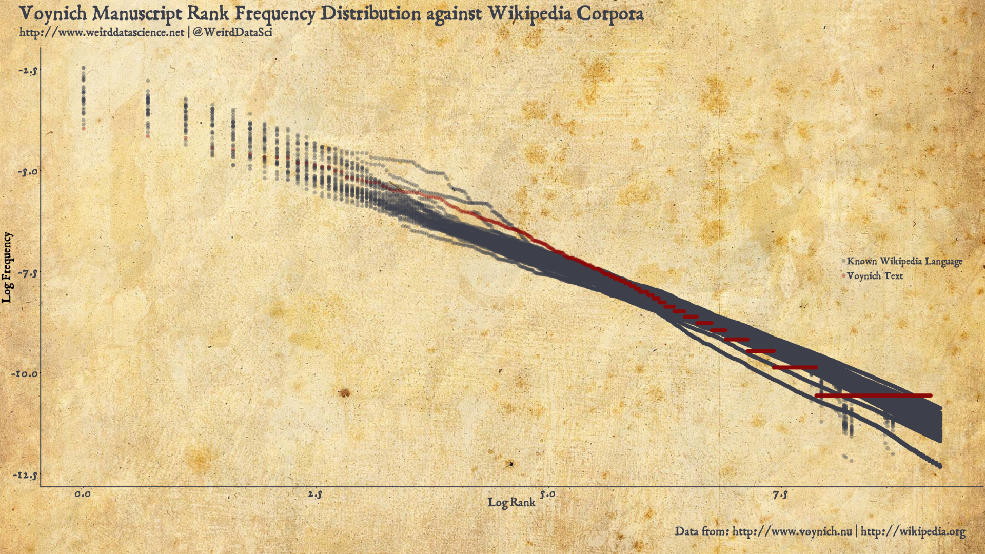
To highlight this phenomenon, we can apply a similar technique to another widely-translated short text: the United Nations Declaration of Human Rights.
Voynich Manuscript Rank Frequency Distribution against UNDHR Translations | (PDF Version)
# Tokenize
# (Remove words of 3 letters or less)
# Stemming and stopword removal apparently not so effective anyway,
# according to Schofield et al.: <www.cs.cornell.edu/~xanda/winlp2017.pdf>
voynich_words <-
voynich_tbl %>%
unnest_tokens( word, text )
# Most common words
message( "Calculating Voynich language statistics…" )
voynich_common <-
voynich_words %>%
count( word, sort=TRUE ) %>%
mutate( word = reorder( word, n ) ) %>%
mutate( freq = n / sum(n) )
# Combine with Voynich, assigning it the unassigned ISO 3166-1 alpha-2 code "vy"
message( "Combining common and Voynich language statistics…" )
voynich_language <-
voynich_common %>%
transmute( language = "vy", freq = freq )
The above arguments might at first appear compelling. The surface incomprehensibility of the Voynich Manuscript succumbs to the deep currents of statistical laws, and reveals an underlying pattern amongst the chaos of the text.
Sadly, however, as with all too many arguments in the literature regarding power law distributions arising in nature, there is a complication to this argument that again highlights the difference between proof and the failure to disprove. Certainly, if a power law had proved incompatible with the Voynich Manuscript then we would have doubted its authenticity. With its apparent adherence to such a distribution, however, we have taken only one hesitant step towards confidence.
Rugg has argued that certain random mechanisms can produce text that adheres to Zipf’s Law, and has demonstrated a simple mechanical procedure for doing so. A more compelling argument is presented, without reference to the Voynich Manuscript, by Li. (1992)2, who demonstrates that a text drawn entirely at random from any given alphabet of symbols that includes a space will result in a text adhering to some form of Zipf-like distribution. We cannot hang our confidence on such a slender thread.
Shifted Parameters
While Zipf’s Law has been shown to hold for human language text, and a text that does not demonstrate it is certainly suspect, it is far from being the only telltale statistical property of natural language. We have already briefly examined sequences of repeated words in the text; we will now delve further.
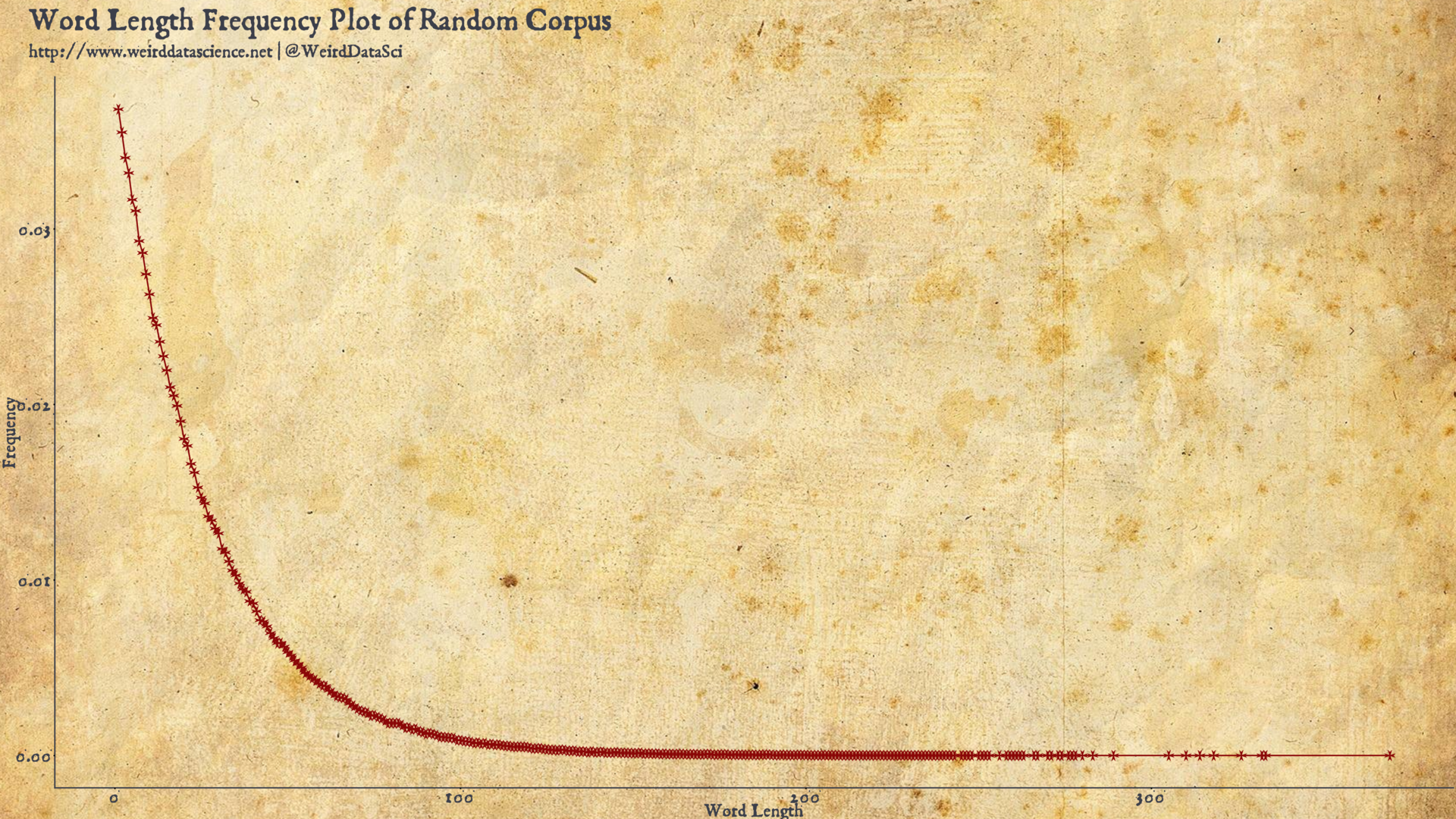
Another curious distortion of human languages is that they demonstrate a preference for shorter words. The precise mechanism that results in this apparently universal property is unclear, but likely relates somehow to efficiency of communication. Regardless of the deeper causality, in most natural language texts there is a markedly higher frequency of short words than longer words.
As demonstrated by Sigurd, Eeg-Olofsson, and van Weijer, (2004)3, however, the very shortest words are not the most common. Instead, at least for English, Swedish, and German, words between 3 and 5 letters in length dominate. This property can be accurately modelled by an appropriately parameterised Gamma distribution.
Notably, and conveniently, this property will not hold for random texts as described above. These purely stochastic texts would be expected to produce, in the long term, a monotonically-decreasing function as word length increases.
To demonstrate this effect, we can simulate a purely random text along the lines discussed by Li, and show its correspondingly naïve descending plot.
Word-Length Frequency Plot of Randomly-Generated Text | (PDF Version)
Word-Length Frequency Plot of Randomly Generated Text
# Vector of symbols (letters) from which to sample.
# Note that a blank space is included as a symbol.
symbol_vector <-
c(
"a","b","c","d","e","f","g","h","i",
"j","k","l","m","n","o","p","q","r",
"s","t","u","v","w","x","y","z"," " )
# Create a corpus of the same number of symbols as our transcription
# of the Voynich Manuscript
random_corpus <-
sample( symbol_vector, size = 16777216, replace = TRUE ) %>%
paste( collapse="" ) %>%
enframe( name=NULL ) %>%
unnest_tokens( word, value )
# Most common words
message( "Calculating word-length frequency statistics…" )
random_length_freq <-
random_corpus %>%
mutate( length = str_length( word ) ) %>%
count( length ) %>%
mutate( freq = n / sum(n) )
# Identify the lengths of words individually as a vector for distribution fitting
random_lengths <-
random_corpus %>%
mutate( length = str_length( word ) ) %>%
extract2( "length" )
# Plot length frequency curve.
gp <-
ggplot( random_length_freq, aes( x = length, y = freq ) ) +
geom_line( colour="#8a0707" ) +
geom_text( colour="#8a0707", label="\u2720", family = "unicode_font", size=4 ) +
labs(
x = "Word Length",
y = "Frequency" )
As can be seen, the word-length frequency of this random text forms a comfortingly simple exponential curve, with pseudo-words of one letter being by far the most common. It is also notable that, at the far reaches of the probability distribution, this cacophonous experiment will produce words of almost four-hundred letters in length. While adherence to Zipf’s Law would have misled us into supporting this as an apparently natural language, even a cursory glance at this plot would have convinced us otherwise.
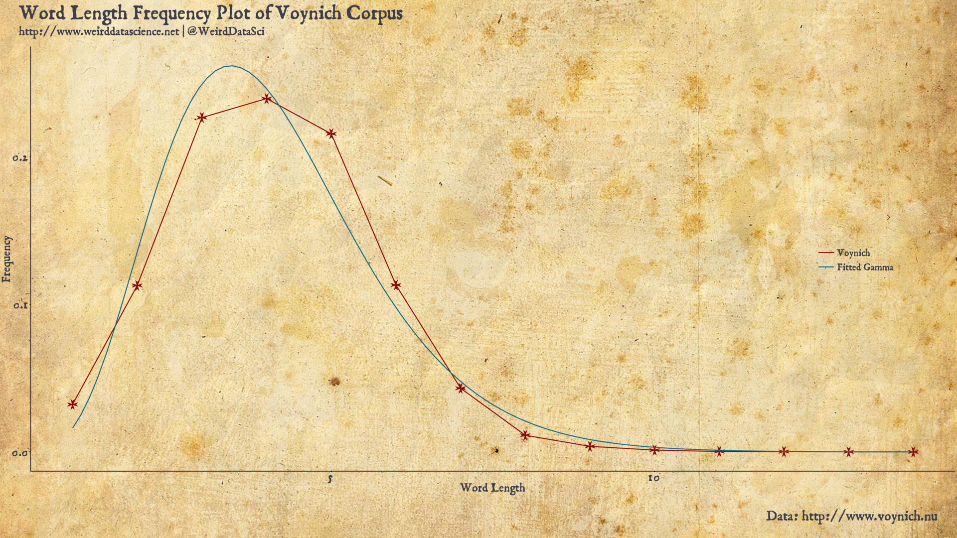
How, then, does the Voynich Manuscript adhere to the expected Gamma distribution of Sigurd et al.? We can employ the excellent fitdistrplus package to peel back this particular veil.
Voynich Word-Length Frequency with Fitted Gamma Distribution | (PDF Version)
The word-length frequency distribution of the Voynich Manuscript clearly demonstrates a preference for four-letter words, not only breaking free of the confines of pure randomness, but also corresponding broadly with observed frequency patterns of the languages tested by Sigurd et al.
Fitting Gamma distribution to Voynich Manuscript corpus
# Tokenize
voynich_words <-
voynich_tbl %>%
unnest_tokens( word, text )
# Most common words
message( "Calculating Voynich language word-length frequency statistics…" )
voynich_length_freq <-
voynich_words %>%
mutate( length = str_length( word ) ) %>%
count( length ) %>%
mutate( freq = n / sum(n) )
# Identify the lengths of words individually as a vector for distribution fitting
voynich_lengths <-
voynich_words %>%
mutate( length = str_length( word ) ) %>%
extract2( "length" )
# Fit a gamma distribution to the observed frequencies
# Extract frequency counts for lengths
gamma_fit <-
fitdist( voynich_lengths, "gamma" )
# Plot length frequency curve.
gp <-
ggplot( voynich_length_freq, aes( x = length, y = freq ) ) +
geom_line( aes( colour="Voynich" ) ) +
geom_text( colour="#8a0707", label="\u2720", family = "unicode_font", size=6 ) +
labs(
x = "Word Length",
y = "Frequency" )
# Overlay fitted gamma distribution
gp <-
gp +
stat_function(
fun=dgamma,
args=list(
shape = gamma_fit$estimate["shape"],
rate = gamma_fit$estimate["rate"] ),
aes( colour = "Fitted Gamma" ) )
# Label gamma line and original data.
# (The ‘breaks’ argument to scale_colour_manual reorders the lines manually,
# otherwise they will be ordered alphabetically. This is useful for combined
# plots where there isn’t a colour factor variable that can be reordered.)
gp <-
gp +
scale_colour_manual(
values = c("Fitted Gamma" = "#0b6788", "Voynich" = "#8a0707" ),
breaks = c("Voynich", "Fitted Gamma" )
)
These analyses can only present a dim outline of the text itself, and we resist the awful temptation to attempt any form of decipherment. Certainly, the evidence here seems convincing enough that the Voynich Manuscript does represent a human language, but the statistics presented here are of little use in such an effort. It is likely, of course, that the most frequent words in the manuscript may, under certain assumptions, correspond to the most common words or particles in many languages — the definite article, the indefinite article, conjunctions, pronouns, and similar. Without deeper knowledge of the language, however, and with the range of scribing conventions and shortcuts commonplace in texts of the period, these techniques are too limited to do more than tantalise us with what we may never know.
Credible Conclusions
Subjecting the text of the Voynich Manuscript to the crude frequency analyses presented here can support, although not prove, the view that the manuscript, regardless of its true content, is not simply random gibberish. Nor is the text likely to be the result of a simple mechanical process designed without knowledge of the statistical patterns of human languages. Neither is it likely to be any form of cryptogram more sophisticated than the simplest ciphers, as these would have tended to compromise the statistical properties that we have observed.
The demonstrable following of Zipf’s Law, and the adherence to a Gamma distribution of similar shape to known languages, strongly suggests that the text is likely a representation of some natural language.
In the next post we will attempt blindly to wrench more secrets from the text itself through application of modern textual analysis techniques. Until then the Voynich Manuscript remains, silently obscure, beyond the reach of our faltering science.
Footnotes
The distributions observed in natural languages are therefore best described as following several parameterisations of the slightly more complex, generalised Zipf–Mandelbrot distribution, with different parameters for the most common, middle, and least-common segments of the corpus.
Li, W. ‘Random Texts Exhibit Zipf’s-Law-like Word Frequency Distribution’. IEEE Transactions on Information Theory 38, no. 6 (November 1992): 1842–45. https://doi.org/10.1109/18.165464.
Sigurd, Bengt, Mats Eeg-Olofsson, and Joost van Weijer. ‘Word Length, Sentence Length and Frequency – Zipf Revisited’. Studia Linguistica 58, no. 1 (April 2004): 37–52. https://doi.org/10.1111/j.0039-3193.2004.00109.x.

Be the first to comment
This site uses User Verification plugin to reduce spam. See how your comment data is processed.