Sealed and Buried

In the previous three posts¹ in our series delving into the cosmic horror of UFO sightings in the US, we have descended from the deceptively warm and sunlit waters of basic linear regression, through the increasingly frigid, stygian depths of Bayesian inference, generalised linear models, and the probabilistic programming language Stan.

In this final post we will explore the implications of the murky realms in which we find ourselves, and consider the awful choices that have led us to this point. We will therefore look, with merciful brevity, at the foul truth revealed by our models, but also consider the arcane philosophies that lie sleeping beneath.

Deviant Interpretations

Our crazed wanderings through dark statistical realms have led us eventually to a varying slope, varying intercept negative binomial generalised linear model, whose selection was justified over its simpler cousins via leave-one-out cross-validation (LOO-CV). By interrogating the range of hyperparameters of this model, we could reproduce an alluringly satisfying visual display of the posterior predictive distribution across the United States:

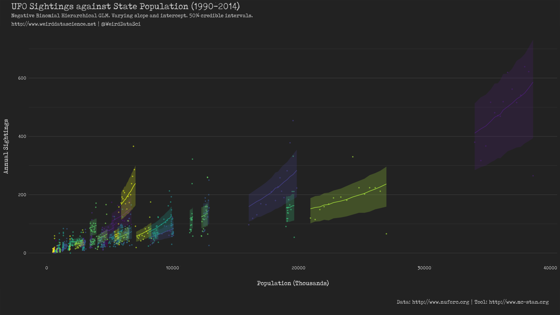
Varying intercept and slope negative binomial GLM of UFO sightings against population. (PDF Version)

Further, our model provides us with insight into the individual per-state intercept $\alpha$ and slope $\beta$ parameters of the underlying linear model, demonstrating that there is variation between the rate of sightings in US states that cannot be accounted for by their ostensibly human population.

Varying slope and intercept negative binomial GLM parameter plot for UFO sightings model. (PDF Version)

Interpreting these parameters, however, is not as quite as simple as in a basic linear model². Most importantly our negative binomial GLM employs a log link function to relate the linear model to the data:

$$\begin{eqnarray}
y &\sim& \mathbf{NegBinomial}(\mu, \phi)\\
\log(\mu) &=& \alpha + \beta x\\
\alpha &\sim& \mathcal{N}(0, 1)\\
\beta &\sim& \mathcal{N}(0, 1)\\
\phi &\sim& \mathbf{HalfCauchy}(2)
\end{eqnarray}$$

In a basic linear regression, $y=\alpha+\beta x$, the $\alpha$ parameter can be interpreted as the value of $y$ when $x$ is 0. Increasing the value of $x$ by 1 results in a change in the $y$ value of $\beta$. We have, however, been drawn far beyond such naive certainties.

The $\alpha$ and $\beta$ coefficients in our negative binomial GLM produce the $\log$ of the $y$ value: the mean of the negative binomial in our parameterisation.

With a simple rearrangement, we can being to understand the grim effects of this transformation:

$$\begin{array}
_ & \log(\mu) &=& \alpha + \beta x\\
\Rightarrow &\mu &=& \operatorname{e}^{\alpha + \beta x}\\
\end{array}$$

If we set $x=0$:

$$\begin{eqnarray}
\mu_0 &=& \operatorname{e}^{\alpha}
\end{eqnarray}$$

The mean of the negative binomial when $x$ is 0 is therefore $\operatorname{e}^{\alpha}$. If we increase the value of $x$ by 1:

$$\begin{eqnarray}
\mu_1 &=& \operatorname{e}^{\alpha + \beta}\\
&=& \operatorname{e}^{\alpha} \operatorname{e}^{\beta}
\end{eqnarray}$$

Which, if we recall the definition of the underlying mean of our model’s negative binomial, $\mu_0$, above, is:
$$\mu_0 \operatorname{e}^{\beta}$$

The effect of an increase in $x$ is therefore multiplicative with a log link: each increase of $x$ by 1 causes the mean of the negative binomial to be further multiplied by $\operatorname{e}^{\beta}$.

Despite this insidious complexity, in many senses our naive interpretation of these values still holds true. A higher value for the $\beta$ coefficient does mean that the rate of sightings increases more swiftly with population.

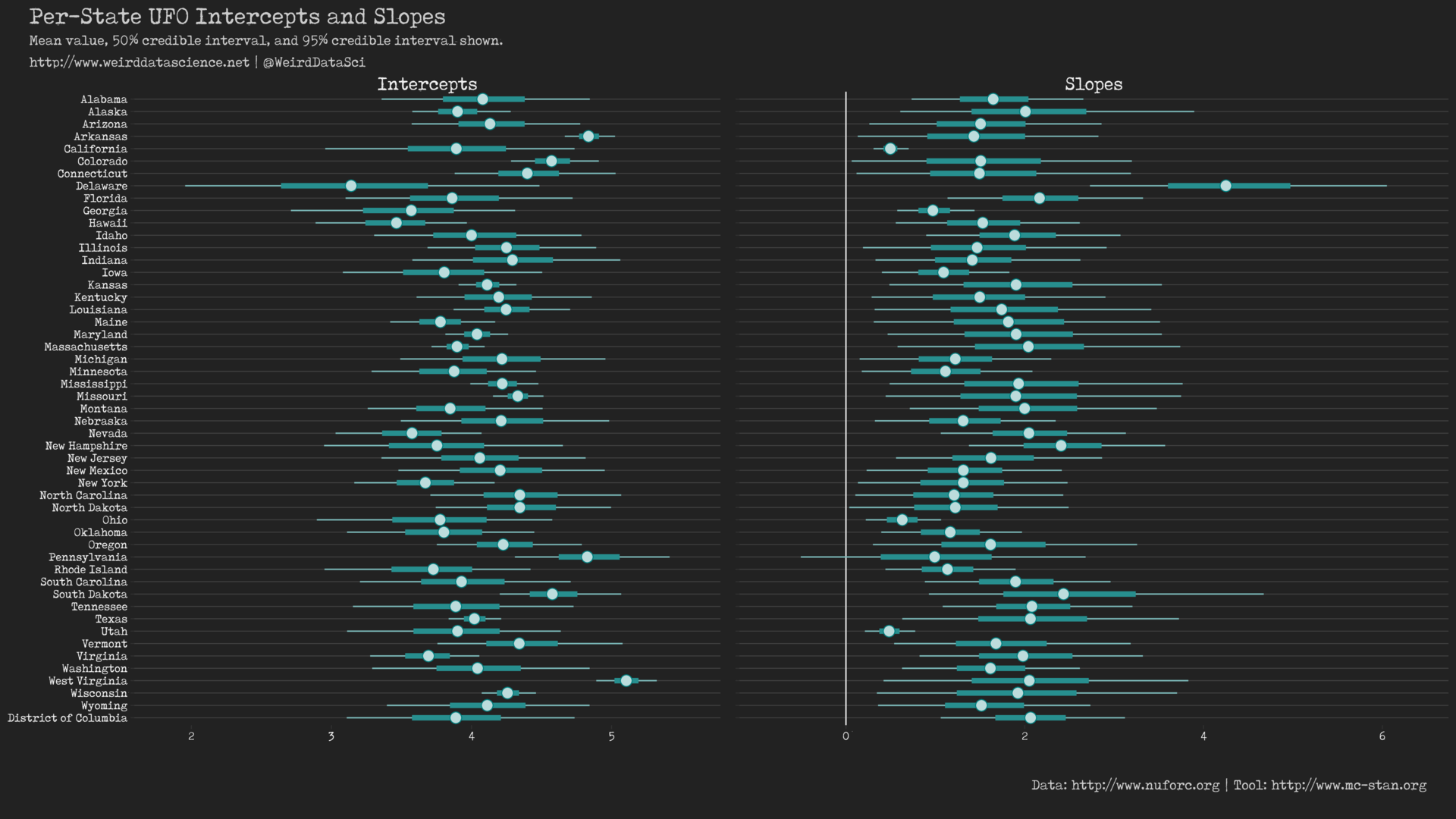
With the full, unsettling panoply of US States laid out before us, any attempt to elucidate their many and varied deviations would be overwhelming. Broadly, we can see that both slope and intercepts are generally restricted to a fairly close range, with the 50% and 95% credible intervals notably overlapping in many cases. Despite this, there are certain unavoidable abnormalities from which we cannot, must not, shrink:

Only Pennsylvania presents a slope ($\beta$) parameter that could be considered as potentially zero, if we consider its 95% credible interval. The correlation between population and number of sightings is otherwise unambiguously positive.
Delaware, whilst presenting a wide credible interval for its slope ($\beta$) parameter, stands out as suffering from the greatest rate of change in sightings as its population increases.
Both California and Utah, present suspiciously narrow credible intervals on their slope ($\beta$) parameters. The growth in sightings as the population increases therefore demonstrates a worrying consistency although, in both cases, this rate is amongst the lowest of all the states.

We can conclude, then, that while the total number of sightings in Delaware are currently low, any increase in numbers of residents there appears to possess a strange fascination for visitors from beyond the inky blackness of space. By contrast, whilst our alien observers have devoted significant resources to monitoring Utah and California, their apparent willingness to devote further effort to tracking those states’ burgeoning populations is low.

Trembling Uncertainty

One of the fundamental elements of the Bayesian approach is its willing embrace of uncertainty. The output of our eldritch inferential processes are not point estimates of the outcome, as in certain other approaches, but instead posterior predictive distributions for those outcomes. As such, if when we turn our minds to predicting new outcomes based on previously unseen data, our outcome is a distribution over possible values rather than a single estimate. Thus, at the dark heart of Bayesian inference is a belief in the truth that all uncertainty be quantified as probability distributions.

The Bayesian approach as inculcated here has a predictive bent to it. These intricate methods lend themselves to forecasting a distribution of possibilities before the future unveils itself. Here, we gain a horrifying glimpse into the emerging occurrence of alien visitations to the US as its people busy themselves about their various concerns, scrutinised and studied, perhaps almost as narrowly as a man with a microscope might scrutinise the transient creatures that swarm and multiply in a drop of water.

Unavoidable Choices

The twisted reasoning underlying this series of posts has been not only in indoctrinating others into the hideous formalities of Bayesian inference, probabilistic programming, and the arcane subtleties of the Stan programming language; but also as an exercise in exposing our own minds to their horrors. As such, there is a tentative method to the madness of some of the choices made in this series that we will now elucidate.

Perhaps the most jarring choice has been to code these models in Stan directly, rather than using one of the excellent helper libraries that allow for more concise generation of the underlying Stan code. Both brms and rstanarm possess the capacity to spawn models such as ours with greater simplicity of specification and efficiency of output, due to a number of arcane tricks. As an exercise in internalising such forbidden knowledge, however, it is useful to address reality unshielded by such swaddling conveniences.

In fabricating models for more practical reasons, however, we would naturally turn to these tools unless our unspeakable demands go beyond their natural scope. As a personal choice, brms is appealing due to its more natural construction of readable per-model Stan code to be compiled. This allows for the grotesque internals of generated models to be inspected and, if required, twisted to whatever form we desire. rstanarm, by contrast, avoids per-model compilation by pre-compiling more generically applicable models, but its underlying Stan code is correspondingly more arcane for an unskilled neophyte.

The Stan models presented in previous posts have also been constructed as simply as possible and have avoided all but the most universally accepted tricks for improving speed and stability³. Most notably, Stan presents specific functions for GLMs based on the Poisson and negative binomial distributions that apply standard link functions directly. As mentioned, we consider it more useful for personal and public indoctrination to use the basic, albeit log-form parameterisations.

Last Rites

In concluding the dark descent of this series of posts on Bayesian inference, generalised linear models, and the unearthly effects of extraterrestrial visitions on humanity, we have applied numerous esoteric techniques to identify, describe, and quantify the relationship between human population and UFO sightings. The enigmatic model constructed throughout this and the previous three entries darkly implies that, while the rate of inexplicable aerial phenomena is inextricably and positively linked to humanity’s unchecked growth, there are nonetheless unseen factors that draw our non-terrestrial visitors to certain populations more than others, and that their focus and attention is ever more acute.

This series has inevitably fallen short of a full and meaningful elucidation of the techniques of Bayesian inference and Stan. From this first step on such a path, then, interested students of the bizarre and arcane would be well advised to draw on the following esoteric resources:

Until then, watch the skies and archive your data.

Footnotes

To immerse yourself in the full horror of our journey, the previous posts in this series are here:
One advantage of generalised linear models is that they allow flexibility whilst remaining relatively interpretable. As models become more complex, extending generalised linear models (GLMs) through generalised additive models (GAMs), and further into the vast chaotic mass of machine learning approaches such as random forests and convolutional neural networks, there is a general tradeoff between the terrifying power of the modelling technique and the ability of the human mind to correlate its contents.
The most important of these are to center and scale our predictors, and to operate on the log scale through use of the log form of the probability distribution sampling statements. Both of these contribute significantly to speed and numerical stability in sampling, and are sufficiently universal that their inclusion seemed justified.

Bayes vs. the Invaders! Part Four: Convergence