Missing Links: Density of Bigfoot Sightings in North America

Sightings of Homo sapiens cognatus, or Homo sylvestris, are well-recorded, with a particular prevalence in North America. Bigfoot, otherwise known as the Sasquatch, is one of the most widely-reported cryptids in the world; it is the subject of documentaries, film, music, and countless books.

The Bigfoot Field Research Organisation has compiled a detailed database of Bigfoot sightings going back to the 1920s. Each sighting is dated, located to the nearest town or road, and contains a full description of the sighting. In many cases, sightings are accompanied by a follow-up report from the organisation itself.

As previously with UFO sightings and paranormal manifestations, our first step is to retrieve the data and parse it for analysis. Thankfully, the bfro.net dataset is relatively well-formatted; reports are broken down by region, with each report following a mainly standard format.

As before, we rely on the rvest package in R to explore and scrape the website. In this case, the key elements were to retrieve each state’s set of reports from the top level page, and retrieve the link for each report. Conveniently, these are in a standard format; the website also allows a printer-friendly mode that greatly simplifies scraping.

The scraping code is given here:

Show scraping code.

[code language=”r”]

library(tidyverse)
library(progress)
library(rvest)

# Base URLs for scraping
index_url <- "https://www.bfro.net/GDB/"
base_url <- "https://www.bfro.net"
report_base_url_pattern <- "https:\\/\\/www.bfro.net\\/GDB\\/show_report.asp\\?id="

# Retrieve list of state-level county report pages
get_state_listing_urls <- function( url ) {

read_html( url ) %>%
html_nodes( ‘a’ ) %>%
html_attr( ‘href’ ) %>%
str_match( ‘.*state_listing.asp\\?state=.*’ ) %>%
na.omit %>%
unique %>%
{ paste0( base_url, . ) }

}

# Return all URLs pointing to a county-level list of reports
get_county_report_urls <- function( url ) {

read_html( url ) %>%
html_nodes( ‘a’ ) %>%
html_attr( ‘href’ ) %>%
str_match( ‘.*show_county_reports.asp\\?state=.*’ ) %>%
na.omit %>%
unique %>%
{ paste0( index_url, . ) }

}

# Return all URLs pointing to a report in this page.
get_report_urls <- function( url ) {

read_html( url ) %>%
html_nodes( ‘a’ ) %>%
html_attr( ‘href’ ) %>%
str_match( ‘.*show_report.asp\\?id=[0-9]+’ ) %>%
na.omit %>%
unique %>%
{ paste0( index_url, . ) }

}

progressive_get_county_report_urls <- function( url, progress_bar ) {

progress_bar$tick()$print()
cat( paste(url, "\n") , file="work/progress.log", append=TRUE )
chime()
get_county_report_urls( url )

}

progressive_get_report_urls <- function( url, progress_bar ) {

progress_bar$tick()$print()
cat( paste(url, "\n") , file="work/progress.log", append=TRUE )
get_report_urls( url )

}

# Pull the report listing from a page.
store_report <- function( url ) {

report_id <-
url %>%
str_replace( report_base_url_pattern, "" ) %>%
str_replace( "/", "-" ) %>%
str_replace( ".html", "" )

#message( paste0("Processing report ", report_id, "… " ), appendLF=FALSE )

# Check if this report has already been stored.
if( file.exists( paste0( "data/", report_id, ".rds" ) ) ) {
message( paste0( "Report already retrieved: ", report_id ) )
return()
}

url_pf <- paste0( url, "&PrinterFriendly=True" )

report <-
tryCatch(
{
# Fetch and parse HTML of current page.
read_html( url_pf ) %>%
as.character
},
error=function( cond ) {
message( paste( "URL caused an error:", url ))
message( "Error message:")
message( cond )
return( NULL )
},
warning=function( cond ) {
message( paste( "URL caused a warning:", url ))
message( "Warning message:")
message( cond )
return( NULL )
},
finally={
}
)

# Write report result to disk
saveRDS( report, paste0("data/", report_id, ".rds") )

}

# Progressive version of store_report
progressive_store_report <- function( url, progress_bar ) {

progress_bar$tick()$print()
cat( paste(url, "\n") , file="work/progress.log", append=TRUE )
store_report( url )

}

# The key to this is that links of the form
# <https://www.bfro.net/GDB/show_county_reports.asp?state=…>
# link to each state’s data. At the top level, then, we can just get all links matching that form.

# At each sub-page, the links are:
# <https://www.bfro.net/GDB/show_report.asp?id=…>
# We can just pull all of those for each state.
# NOTE: There are also non-US reports linked like this directly from the main GDB page.

# Finally, it seems that adding "&PrinterFriendly=True" will strip a lot of
# unnecessary formatting.

# From the top-level page, get every URL that matches ‘show_county_reports.asp?state=’, make
# the list unique, then download the pages.

# Get all non-US state indices
message("Getting state report lists…", appendLF=FALSE )
bfro_state_indices <- get_state_listing_urls( index_url )
message("done." )
saveRDS( bfro_state_indices, "work/bfro_state_indices.rds" )

# Get all US county-level indices
message("Getting county-level report urls… " )
pb <- progress_estimated( length( bfro_state_indices ) )
bfro_county_urls <-
bfro_state_indices %>%
map( progressive_get_county_report_urls, pb ) %>%
unlist %>%
unique
saveRDS( bfro_county_urls, "work/bfro_county_urls.rds" )

# Get URLs of US reports from county pages.
# (Final subset line handles cases where pages are empty of reports, but
# contain other links such as media articles.)
pb <- progress_estimated( length( bfro_county_urls ) )
bfro_report_urls <-
bfro_county_urls %>%
map( progressive_get_report_urls, pb ) %>%
unlist %>%
unique %>%
str_subset( "GDB\\/." )
saveRDS( bfro_report_urls, "work/bfro_report_urls.rds" )

# Store all US reports
pb <- progress_estimated( length( bfro_report_urls ) )
bfro_report_urls %>%
map( progressive_store_report, pb )

# Get all non-US indices
message("Getting non-US top-level report lists…", appendLF=FALSE )
bfro_nonus_indices <-
get_county_report_urls( index_url ) %>%
str_replace( "GDB\\/\\/", "\\/" )
message("done." )
saveRDS( bfro_nonus_indices, "work/bfro_nonus_indices.rds" )

# Get URLs of US reports from county pages
message("Getting non-US report lists…", appendLF=FALSE )
pb <- progress_estimated( length( bfro_nonus_indices ) )
bfro_nonus_report_urls <-
bfro_nonus_indices %>%
map( progressive_get_report_urls, pb ) %>%
unlist %>%
unique %>%
str_subset( "GDB\\/." )
saveRDS( bfro_nonus_report_urls, "work/bfro_nonus_report_urls.rds" )

# Store all US reports
pb <- progress_estimated( length( bfro_nonus_report_urls ) )
bfro_nonus_report_urls %>%
map( progressive_store_report, pb )

[/code]

With each page retrieved, we step through and parse each report. Again, each page is fairly well-formatted, and uses a standard set of tags for date, location, and similar. The report parsing code is given here:

Show parsing code.

[code language=”r”]

# NOTES

# Process entire list to check for standardised headers. These are in capitals, and located in tags.

# Report starts with:
# 
# (Look up what these mean.)
# Some following types contain general summary information, eg:
# " Submitted by witness on Thursday, November 1, 2007."
# Following fields are in span tags separated by paragraph tags, eg:
# YEAR: 2007
# STATE and COUNTY fields are typically links; we should pull their text. (I can’t see a good reason to parse links to anything other than the link text for our purposes.)

library(tidyverse)
library(magrittr)
library(progress)
library(rvest)
library(lubridate)

# Exploratory functions

# List all capitalised fields seen in any file
list_all_fields <- function() {

filenames <- list.files( "data", pattern="*.rds", full.names=TRUE)

# In each file, select the classes, match the uppercase field names, and extract text.
all_fields <-
filenames %>%
map( list_report_fields ) %>%
unlist %>%
unique

saveRDS( all_fields, "work/fields.rds" )

return( all_fields )

}

fields_to_colnames <- function( fields ) {

# In total there are 18 fields reported in the data, with the final one
# being an apparently miscoded date and place from a report.

# Format the text appropriately for dataframe column names
fields %>%
head( 17 ) %>%
str_remove( ":" ) %>%
str_replace_all( " ", "_" ) %>%
str_to_lower()

}

list_report_fields <- function( report ) {

to_process <- readRDS( report )

bfro_fields <- NULL

if( !is.null( to_process ) ) {
bfro_fields <-
to_process %>%
read_html %>%
html_nodes( "span" ) %>%
html_nodes(xpath = ‘//*[@class="field"]’) %>%
html_text %>%
str_subset( "[A-Z]+:" )
}

return( bfro_fields )
}

# Extract node date
parse_report_data <- function( report_data ) {

# report_data should be an xml_nodeset

# Metadata
metadata_list <-
report_data %>%
html_text %>%
str_subset( "^[A-Z ]+: " ) %>%
str_split_fixed( ": ", 2 ) %>%
as.tibble %>%
spread( key=V1, value=V2 ) %>%
set_colnames( fields_to_colnames( colnames(.) ) )

# Extra details
extra_text <-
report_data %>%
html_text %>%
str_remove( "^[A-Z ]+:.*" ) %>%
str_flatten( " " ) %>%
str_trim

# Add extra details as a column
metadata_list$extra <- extra_text

# Note whether date is rough or accurately reported
metadata_list$rough_date <- FALSE

# "Fix" missing date or month columns
if( "date" %in% colnames( metadata_list ) == FALSE ) {
metadata_list$date <- "1"
metadata_list$rough_date <- TRUE
}

if( "month" %in% colnames( metadata_list ) == FALSE ) {
metadata_list$month <- "January"
metadata_list$rough_date <- TRUE
}

# Combine date columns (year, month, date) to a true date.
metadata_list <-
metadata_list %>%
mutate( year = str_replace( year, ".*([0-9]{4}).*", "\\1" ) ) %>%
mutate( date = paste0( year, "-", month, "-", date ), year=NULL, month=NULL ) %>%
mutate( date = as.POSIXct( date, format="%Y-%B-%d" ) )

}

# Read a file and pass to `post_get_all_thread`
process_file <- function( filename ) {

# Read stored file
to_process <- readRDS( filename )

# Don’t process null files
if( is.null( to_process ) )
return( NULL )

if( length( to_process ) == 0 )
return( NULL )

# Produce an xml_nodeset for parsing
xml_thread <-
to_process %>%
read_html %>%
html_nodes( "p" )

parse_report_data( xml_thread )

}

# Progressive version of process_file
progressive_process_file <- function( filename, progress_bar ) {

progress_bar$tick()$print()
cat( paste(filename, "\n") , file="progress.log", append=TRUE )

report <-
tryCatch(
{
process_file( filename )
},
error=function( cond ) {
message( paste( "File caused an error:", filename ))
message( "Error message:")
message( cond )
return( NULL )
},
warning=function( cond ) {
message( paste( "URL caused a warning:", url ))
message( "Warning message:")
message( cond )
return( NULL )
},
finally={
}
)

return( report )

}

## Processing starts here

# Read all .rds data files and process into a thread
filenames <- list.files("data", pattern="*.rds", full.names=TRUE)
pb <- progress_estimated( length( filenames ) )

# Begin logging
cat( "Processing… ", file="progress.log", append=FALSE )

bfro_tbl <-
filenames %>%
map( progressive_process_file, pb ) %>%
bind_rows

saveRDS( bfro_tbl, "data/bfro_processed.rds" )

[/code]

With each report parsed into a form suitable for analysis, the final step in scraping the site is to geolocate the reports. As in previous posts, we rely on Google’s geolocation API. For each report, we extract an appropriate address and parse it into a set of latitude and longitude coordinates. For the purposes of this initial scrape we restrict ourselves to North America, which compromises a large majority of reports on bfro.net. Geolocation code is included below. (Note that a Google Geolocation API key is required for this code to run.)

Show geolocation code.

[code language=”r”]

library(googleway)
library(progress)
library(tidyverse)
library(magrittr)

# weird.data.science Google API key (Geocoding API enabled)
key <- <INSERT API KEY HERE>

# Load bfro tibble
bfro_data <- readRDS( "data/bfro_processed.rds" )

# Geocode entries

# BFRO entries contain some, all, or none of:
# country, province, state, county, nearest_town

# Country is only used for Canada, in which case a province is given.
# Country and province are NA for the US.

# Best plan, then is to create a string of (nearest_town, province, country) for Canadian results, and (nearest_town, county, state, "US") for US results.

# Bound the request to be only in North America.
# (Used: <https://boundingbox.klokantech.com>)
# (SW->NE latitude and longitude.)
bounding_box <- list( c( -170.3, 24.4),
c( -52.3, 83.3) )

form_location_string <- function( country, province, state, county, nearest_town ) {

location_string <- NA

# US case, then Canadian
if( is.na( country ) )
location_string <- paste0( nearest_town, ", ", county, ", ", state, ", US" )
else
location_string <- paste0( nearest_town, ", ", province, ", ", ", Canada" )

# Strip double commas caused by NA values and remove bracketed clauses.
location_string %<>%
str_remove_all( "\$[^\$]*\\)" ) %>%
str_replace_all( ", , ", ", " ) %>%
str_replace_all( " ,", "," ) %>%
str_remove_all( "NA, " )

}

# Create a safe version of google_geocode
safe_geocode <- safely( google_geocode )

# Wrap google_geocode with a progress bar call.
# Also, optionally remove any bracketed substrings entirely (strip_brackets)
progressive_geocode <- function( location_string, progress_bar ) {

# Write status to log file.
progress_bar$tick()$print()

cat( paste0( location_string, "\n" ), file="progress.log", append=TRUE )

result <-
safe_geocode(
address = location_string,
key = key,
bounds = bounding_box,
simplify = TRUE )

# Note that this can be NULL
return( result$result )

}

# Logging and output
## Clear the screen first
cat(c("\033[2J","\033[0;0H"))
cat("Geolocating entries…\n")
cat( "Geolocating entries…\n", file="progress.log", append=FALSE )

# Create the location string
bfro_data %<>%
mutate( location = form_location_string( country, province, state, county, nearest_town ) )

# Geolocate each location.
pb <- progress_estimated(nrow(bfro_data))
bfro_data$geolocation <-
map( bfro_data$location, progressive_geocode, progress_bar = pb )

cat("\nComplete.\n")

## With all values scraped, save geolocated data.
saveRDS( bfro_data, file="work/bfro_data_geolocated.rds")

[/code]

With geolocated data in hand, we can now venture into the wilds. In which areas of North America are Sasquatch most commonly seen to roam? The plot below shows the overall density of Bigfoot sightings, with individual reports marked.

Density plot of Bigfoot sightings in North America — Density of Bigfoot sightings in North America. (PDF Version)

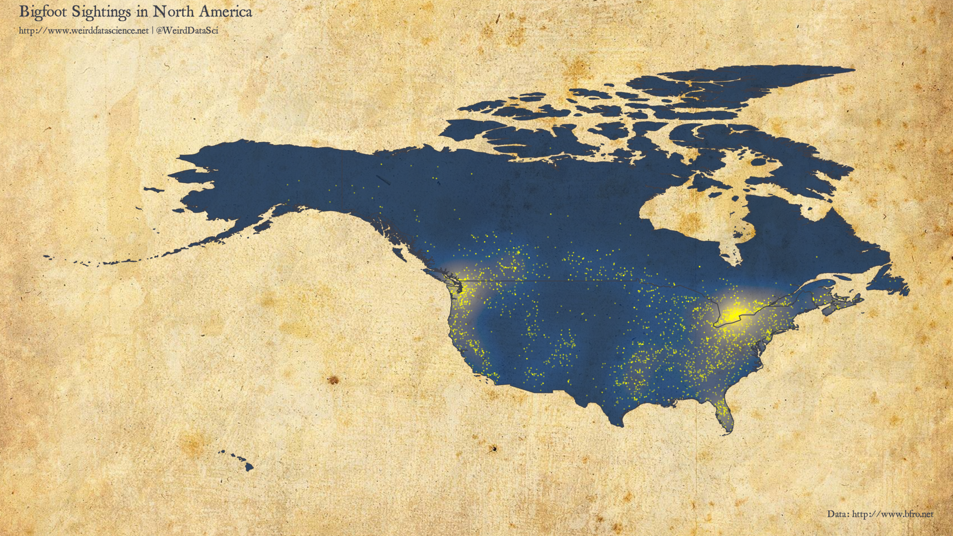
There are particular clusters on the Great Lakes, particularly in Southern Ontario; as well as in the Pacific Northwest. Smaller notable clusters exist in Florida, centered around Orlando. As with most report-based datasets, sightings are skewed towards areas of high population density.

The obvious first question to ask of such data is which, if any, environmental features correlate with these sightings. Other analyses of Bigfoot sightings, such as the seminal work of Lozier et al.¹, have suggested that forested regions are natural habitats for Sasquatch.

To answer this, we combine the underlying mapping data and Bigfoot sightings, with bioclimatic data taken from the Global Land Cover Facility. Amongst other datasets, this provides us with an accurate, high-resolution land cover raster map, detailing vegetation for each 5-arcminute cell in the country — approximately one cell per 10km² .

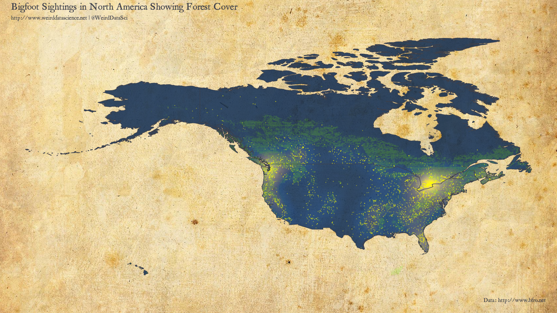
There are a range of bioclimatic variables in this dataset. The diagram below overlays all areas that are some form of forest onto the previous density plot.

Density plot of Bigfoot sightings showing forest cover — Density of Bigfoot sightings in North America (yellow) with forested areas overlaid (green). (PDF Version)

The code for producing both of the above plots is given here:

Show density plotting code.

[code language=”r”]

library(spatstat)

library(rgdal)
library(maptools)

library(tidyverse)
library(magrittr)
library(ggplot2)
library(ggthemes)
library(raster)
library(viridis)
library(scales)

library(sf)

library(showtext)

library(grid)

library(cowplot)
library(magick)

# Load font
font_add( "mapfont", "/usr/share/fonts/TTF/weird/alchemy/1689 GLC Garamond Pro/1689GLCGaramondProNormal.otf" )
showtext_auto()

# Read world shapefile data and tranform to an appropriate projection.
world <- readOGR( dsn=’data/ne/10m_cultural’, layer=’ne_10m_admin_0_countries’ )
world_subset <- world[ world$iso_a2 %in% c("US","CA"), ] world_subset <- spTransform(world_subset,CRS("+init=epsg:4326 +lon_wrap=170"))
world_df <- fortify( world_subset )

# Read bfro database, filtering out locations with "NA" latitude or longitude.
# Also filter results that have been geolocated to "56.13037, -106.3468", which is the centroid of Canada, and results from locations having no more specific result.
bfro_tbl <-
readRDS( "data/bfro_locations.rds" ) %>%
filter( !is.na( lat ) & !is.na( lng ) ) %>%
filter( not( lat == modal( lat ) & lng == modal( lng ) ) )

# Convert the bfro dataframe to a spatial dataframe that contains
# explicit longitude and latitude projected appropriately for plotting.
coordinates( bfro_tbl ) <- ~lng+lat
proj4string( bfro_tbl ) <- CRS("+init=epsg:4326 +lon_wrap=170")
bfro_tbl_spatial <- spTransform(bfro_tbl,CRS(proj4string(bfro_tbl)))

# Restrict bfro_tbl to those points in the polygons defined by world_subset
bfro_tbl_rows <- bfro_tbl_spatial %>%
over( world_subset ) %>%
is.na() %>%
not() %>%
rowSums() %>%
`!=`(0) %>%
which

bfro_tbl <- as.tibble( bfro_tbl_spatial[ bfro_tbl_rows, ] )

# Create window for spatial analysis
bfro_owin <- as.owin.SpatialPolygons(world_subset)

# Function to plot density of a specific manifestation type.
# plot_resolution is for the density raster, and is mainly used for quick prototyping of the output.
density_plot <- function( density_res ) {

cat( paste0( "Plotting density: … " ) )

bfro_ppp <-
ppp(
x=coordinates(bfro_tbl_spatial)[,1],
y=coordinates(bfro_tbl_spatial)[,2],
window = bfro_owin
)

# This discards ‘illegal’ points outside of the window
bfro_ppp <- as.ppp(bfro_ppp)

bfro_density <- density( bfro_ppp, diggle=T, sigma=2, dimyx = c( density_res, density_res ) )

# Make density image object usable by ggplot as a raster
bfro_density_raster <- raster( bfro_density )
bfro_raster_tbl <- as.tibble( rasterToPoints( bfro_density_raster ) )

# Show the map
gp <- ggplot()

# Add density of sightings as raster.
gp <- gp +
geom_raster( data = bfro_raster_tbl, aes( x=x, y=y, fill = layer ), alpha=0.8, show.legend=FALSE ) +
scale_fill_viridis( option = "cividis", direction=1 )

# Add sightings as points.
gp <- gp +
geom_point( data = as.tibble( bfro_ppp ), aes( x=x, y=y ), colour="yellow", size=0.1, alpha=0.5, show.legend=FALSE )

gp <- gp +
geom_map( data = world_df, aes( map_id=id ), colour="#3c3f4a", fill = "transparent", size = 0.4, map = world_df )

# Theming
gp <- gp +
theme_map()

gp <- gp +
theme(
plot.background = element_rect(fill = "transparent", colour = "transparent"),
panel.border = element_blank(),
)

gp <- gp +
guides( fill = guide_colourbar( title.position="top", direction="horizontal", barwidth=6, barheight=0.4 ) )

cat("done.\n" )
return(gp)

}

# Add bioclimatic points to an existing plot
add_bioclimatic_variables <- function( gp, bioclim = seq( 1, 16 ) ) {

# This gets climatic variables for global range.
# (res=0.5 requires latitude and longitude to define a tile to download,
# but 2.5 minutes of a degree is ~5 miles, so probably good enough.)
#wc <- getData( ‘worldclim’, res=2.5, var=’bio’ )

# Value Label
# 0 Water
# 1 Evergreen Needleleaf forest
# 2 Evergreen Broadleaf forest
# 3 Deciduous Needleleaf forest
# 4 Deciduous Broadleaf forest
# 5 Mixed forest
# 6 Closed shrublands
# 7 Open shrublands
# 8 Woody savannas
# 9 Savannas
# 10 Grasslands
# 11 Permanent wetlands
# 12 Croplands
# 13 Urban and built-up
# 14 Cropland/Natural vegetation mosaic
# 15 Snow and ice
# 16 Barren or sparsely vegetated
# 254 Unclassified
# 255 Fill Value

glcf <- raster( "~/opt/datasets/gis/landcover/glcf/LC_5min_global_2012.tif" )

# We can’t just reproject a raster to wrap differently.
# This splits and merges the two edges.
# (This is fragile, unfortunately, but works here.)
# (Reprojecting is best done as the last step, apparently.)
glcf_west <- crop(glcf, extent(-180, 0, 18, 84))
glcf_east <- crop(glcf, extent(0, 180, 18, 84))
extent(glcf_west) <- c(180, 360, 18, 84)
glcf <- merge(glcf_west, glcf_east )

glcf <- crop( glcf, extent( world_subset ) )
glcf <- projectRaster( glcf, crs = CRS("+init=epsg:4326") )

# Make density image object usable by ggplot as a raster
glcf_raster_tbl <- as.tibble( rasterToPoints( glcf ) )
colnames( glcf_raster_tbl ) <- c ("x", "y", "layer" )

# Add bioclimatic variables
gp <- gp +
geom_raster( data = glcf_raster_tbl[ which( glcf_raster_tbl$layer %in% bioclim ), ], alpha=0.8, aes( x=x, y=y ), fill="#7cfc00", show.legend=FALSE )

}

# Cowplot for full-panel plotting. (Parchment background).
theme_set(theme_cowplot(font_size=4, font_family = "mapfont" ) )

# Only calculate the density plot if it isn’t already stored on disk.
if( not( file.exists( "work/density_plot.rds" ) ) ) {
gp <- density_plot( 1024 )
saveRDS( gp, "work/density_plot.rds" )
} else {
gp <- readRDS( "work/density_plot.rds" )
}

# Create a plot including the bioclimatic variables.
bioclim_gp <-
add_bioclimatic_variables( gp, seq( 1, 5 ) )

# Construct full plot, with title and backdrop.
title <- ggdraw() +
draw_label("Bigfoot Sightings in North America", fontfamily="mapfont", colour = "#3c3f4a", size=20, hjust=0, vjust=1, x=0.02, y=0.88) +
draw_label("http://www.weirddatascience.net | @WeirdDataSci", fontfamily="mapfont", colour = "#3c3f4a", size=12, hjust=0, vjust=1, x=0.02, y=0.40)

data_label <- ggdraw() +
draw_label("Data: http://www.bfro.net", fontfamily="mapfont", colour = "#3c3f4a", size=12, hjust=1, x=0.98 )

tgp <- plot_grid(title, gp, data_label, ncol=1, rel_heights=c(0.1, 1, 0.1))

parchment_plot <- ggdraw() +
draw_image("img/parchment.jpg", scale=1.4 ) +
draw_plot(tgp)

save_plot("output/bigfoot-density.pdf",
parchment_plot,
base_width = 16,
base_height = 9,
base_aspect_ratio = 1.78 )

# Add bioclimatic variables to plot.
title <- ggdraw() +
draw_label("Bigfoot Sightings in North America Showing Forest Cover", fontfamily="mapfont", colour = "#3c3f4a", size=20, hjust=0, vjust=1, x=0.02, y=0.88) +
draw_label("http://www.weirddatascience.net | @WeirdDataSci", fontfamily="mapfont", colour = "#3c3f4a", size=12, hjust=0, vjust=1, x=0.02, y=0.40)

data_label <- ggdraw() +
draw_label("Data: http://www.bfro.net", fontfamily="mapfont", colour = "#3c3f4a", size=12, hjust=1, x=0.98 )

tgp <- plot_grid(title, bioclim_gp, data_label, ncol=1, rel_heights=c(0.1, 1, 0.1))

parchment_plot <- ggdraw() +
draw_image("img/parchment.jpg", scale=1.4 ) +
draw_plot(tgp)

save_plot("output/bigfoot-density-forest.pdf",
parchment_plot,
base_width = 16,
base_height = 9,
base_aspect_ratio = 1.78 )

[/code]

From this initial plot we can see that, whilst tree cover is certainly not a bad predictor of Bigfoot sightings, it is far from a definitive correlation. The largest cluster, around the US-Canada border near Toronto, is principally lakes; whilst the secondary cluster in Florida is neither significantly forested or even close to the Everglades, which might have been expected. From the other perspective, there are significant forested areas for which sightings are reasonably rare.

The mystery of Bigfoot’s natural habitat and preferences is, therefore, very much unanswered from our initial analysis. With a broad range of variables still to explore — climate, altitude, food sources — future posts will attempt to determine what conditions lend themselves to strange survivals of pre-human primate activity. Perhaps changing conditions have pushed our far-distant cousins to previously unsuspected regions.

Until then, we keep following these trails into data unknown.

References

Lozier, J. D., Aniello, P. and Hickerson, M. J. (2009), Predicting the distribution of Sasquatch in western North America: anything goes with ecological niche modelling. Journal of Biogeography, 36: 1623-1627. doi:10.1111/j.1365-2699.2009.02152.x (http://onlinelibrary.wiley.com/doi/abs/10.1111/j.1365-2699.2009.02152.x)

Missing Links: Density of Bigfoot Sightings in North America

Be the first to comment

Leave a Reply Cancel reply