Data:
Other:
Combined Plot Code:
[code language=”r”]
library(spatstat)
library(rgdal)
library(maptools)
library(tidyverse)
library(magrittr)
library(ggplot2)
library(ggthemes)
library(raster)
library(viridis)
library(scales)
library(sf)
library(showtext)
library(grid)
library(cowplot)
library(magick)
# Function to combine certain paranormal report types into broader categories
combine_paranormal_types <- function( type ) {
# levels( paranormal_tbl$type )
# [1] "Alien Big Cat" "Crisis Manifestation"
# [3] "Cryptozoology" "Curse"
# [5] "Dragon" "Environmental Manifestation"
# [7] "Experimental Manifestation" "Fairy"
# [9] "Haunting Manifestation" "Legend"
# [11] "Manifestation of the Living" "Other"
# [13] "Poltergeist" "Post-Mortem Manifestation"
# [15] "Shuck" "Spontaneous Human Combustion"
# [17] "UFO" "Unknown Ghost Type"
# [19] "Vampire" "Werewolf"
# Simple lookup
case_when(
type %in% c("Alien Big Cat", "Cryptozoology", "Shuck") ~ "Cryptozoology",
type %in% c("Dragon", "Vampire", "Werewolf" ) ~ "Monster",
type %in% c("Crisis Manifestation", "Environmental Manifestation", "Experimental Manifestation", "Haunting Manifestation", "Manifestation of the Living", "Poltergeist", "Post-Mortem Manifestation", "Unknown Ghost Type") ~ "Haunting",
type %in% c("Legend", "Fairy", "Curse") ~ "Legend",
type %in% c("Spontaneous Human Combustion", "Other") ~ "Other",
type %in% c("UFO") ~ "UFO"
)
}
# Load font
font_add( "mapfont", "/usr/share/fonts/TTF/weird/JANCIENT.TTF" )
showtext_auto()
# Read world shapefile data and tranform to an appropriate projection.
# Limit to the UK, Ireland, and the Isle of Man
world <- readOGR( dsn=’data/ne/10m_cultural’, layer=’ne_10m_admin_0_countries’ )
world_subset <- world[ world$iso_a2 %in% c("GB","IE","IM"), ]
world_subset <- spTransform(world_subset,CRS("+init=epsg:4326"))
world_df <- fortify( world_subset )
# Read paranormal database
paranormal_tbl <- as.tibble( read.csv( file="data/paranormal_database.csv" ) )
# Convert the paranormal dataframe to a spatial dataframe that contains
# explicit longitude and latitude projected appropriately for plotting.
coordinates( paranormal_tbl ) <- ~lng+lat
proj4string( paranormal_tbl )<-CRS("+init=epsg:4326")
paranormal_tbl <- spTransform(paranormal_tbl,CRS(proj4string(paranormal_tbl)))
# Restrict paranormal_tbl to those points in the polygons defined by world_subset
paranormal_tbl_rows <- paranormal_tbl %>%
over( world_subset ) %>%
is.na() %>%
not() %>%
rowSums() %>%
`!=`(0) %>%
which
paranormal_tbl <- as.tibble( paranormal_tbl[ paranormal_tbl_rows, ] )
paranormal_tbl$combined_type <- paranormal_tbl$type %>%
map( combine_paranormal_types ) %>%
unlist
# Show the map
gp <- ggplot() +
geom_map( data = world_df, aes( map_id=id ), colour = "#3c3f4a", fill = "transparent", size = 0.5, map = world_df )
# Display each sighting as geom_point. Use a level of transparency to highlight
# more common areas. (On the 20180401 dataset, this reports that 16035 out of
# the original 19387 points lie in the appropriate area. Several are geolocated
# outside of the UK — the geolocation should be run again with better bounds
# checking and region preference.)
gp <- gp + geom_point(data=paranormal_tbl, aes(x=lng, y=lat, colour=combined_type ), size=0.5, shape=17, alpha=0.9) +
expand_limits(x = world_df$long, y = world_df$lat)
gp <- gp +
# Theming
theme_map() +
theme(
plot.background = element_rect(fill = "transparent", colour = "transparent"),
panel.border = element_blank(),
plot.title = element_text( size=24, colour="#3c3f4a", family="mapfont" ),
text = element_text( size=14, color="#3c3f4a", family="mapfont" ),
) +
theme(
legend.background = element_rect( colour ="transparent", fill = "transparent" ),
legend.key = element_rect(fill = "transparent", colour="transparent"),
legend.position = "left",
legend.justification = c(0,0)
) +
guides( fill = guide_colourbar( title.position="top", direction="vertical", barwidth=32, nrow=1 ) ) +
guides(colour = guide_legend(override.aes = list(size=2)) ) +
scale_colour_manual(
values = c("#00EA38","#417CCC","#B79F00","#F564E3","#00BFC4","#F8766D"),
breaks = c("Haunting", "Cryptozoology", "Monster", "Legend", "UFO", "Other" ),
name = "Manifestation" ) +
coord_fixed( ratio=1.2 )
# Cowplot trick for ggtitle
title <- ggdraw() +
draw_label("Paranormal Manifestations in the British Isles", fontfamily="mapfont", colour = "#3c3f4a", size=24, hjust=0, vjust=1, x=0.02, y=0.88) +
draw_label("http://www.weirddatascience.net | @WeirdDataSci", fontfamily="mapfont", colour = "#3c3f4a", size=14, hjust=0, vjust=1, x=0.02, y=0.40)
data_label <- ggdraw() +
draw_label("Data from: http://www.paranormaldatabase.com", fontfamily="mapfont", colour = "#3c3f4a", size=12, hjust=1, x=0.98 )
paranormal_legend <- get_legend(gp)
# Remove legend from internal plot
gp <- gp + theme(legend.position=’none’)
tgp <- plot_grid(title, gp, data_label, ncol=1, rel_heights=c(0.1, 1, 0.1))
vellum_plot <- ggdraw() +
draw_image("img/vellum.jpg", scale=1.4 ) +
draw_plot(tgp) +
draw_plot( paranormal_legend, 0.02, 0.03 )
save_plot("output/paranormal.pdf",
vellum_plot,
base_width = 16,
base_height = 9,
base_aspect_ratio = 1.78 )
[/code]
Per-Manifestation Density Plot Code:
[code language=”r”]
library(spatstat)
library(rgdal)
library(maptools)
library(tidyverse)
library(magrittr)
library(ggplot2)
library(ggthemes)
library(raster)
library(viridis)
library(scales)
library(sf)
library(showtext)
library(grid)
library(cowplot)
library(magick)
# Function to combine certain paranormal report types into broader categories
combine_paranormal_types <- function( type ) {
# levels( paranormal_tbl$type )
# [1] "Alien Big Cat" "Crisis Manifestation"
# [3] "Cryptozoology" "Curse"
# [5] "Dragon" "Environmental Manifestation"
# [7] "Experimental Manifestation" "Fairy"
# [9] "Haunting Manifestation" "Legend"
# [11] "Manifestation of the Living" "Other"
# [13] "Poltergeist" "Post-Mortem Manifestation"
# [15] "Shuck" "Spontaneous Human Combustion"
# [17] "UFO" "Unknown Ghost Type"
# [19] "Vampire" "Werewolf"
# Simple lookup
case_when(
type %in% c("Alien Big Cat", "Cryptozoology", "Shuck") ~ "Cryptozoology",
type %in% c("Dragon", "Vampire", "Werewolf" ) ~ "Monster",
type %in% c("Crisis Manifestation", "Environmental Manifestation", "Experimental Manifestation", "Haunting Manifestation", "Manifestation of the Living", "Poltergeist", "Post-Mortem Manifestation", "Unknown Ghost Type") ~ "Haunting",
type %in% c("Legend", "Fairy", "Curse") ~ "Legend",
type %in% c("Spontaneous Human Combustion", "Other") ~ "Other Manifestation",
type %in% c("UFO") ~ "UFO"
)
}
# Load font
font_add( "mapfont", "/usr/share/fonts/TTF/weird/JANCIENT.TTF" )
showtext_auto()
# Read world shapefile data and tranform to an appropriate projection.
# Limit to the UK, Ireland, and the Isle of Man
world <- readOGR( dsn=’data/ne/10m_cultural’, layer=’ne_10m_admin_0_countries’ )
world_subset <- world[ world$iso_a2 %in% c("GB","IE", "IM"), ]
world_subset <- spTransform(world_subset,CRS("+init=epsg:4326"))
world_df <- fortify( world_subset )
# Read UK Major Cities datafile
#cities <- readOGR( dsn=’data/ons_uk_cities’, layer=’Major_Towns_and_Cities_December_2015_Boundaries’ )
#cities <- spTransform(cities,CRS("+init=epsg:4326"))
#cities_fortified <- fortify( cities )
#cities_centroids_tbl <- as.tibble( coordinates( cities ) )
#cities_tbl <- as.tibble( cbind( cities@data$tcity15nm, cities_centroids_tbl ))
#colnames(cities_tbl) <- c( "city", "lng", "lat" )
# As the polygons are more confusing than useful, instead label centroids
# Read paranormal database
paranormal_tbl <- as.tibble( read.csv( file="data/paranormal_database.csv" ) )
paranormal_tbl$combined_type <- paranormal_tbl$type %>%
map( combine_paranormal_types ) %>%
unlist
# Convert the paranormal dataframe to a spatial dataframe that contains
# explicit longitude and latitude projected appropriately for plotting.
coordinates( paranormal_tbl ) <- ~lng+lat
proj4string( paranormal_tbl )<-CRS("+init=epsg:4326")
paranormal_tbl_spatial <- spTransform(paranormal_tbl,CRS(proj4string(paranormal_tbl)))
# Restrict paranormal_tbl to those points in the polygons defined by world_subset
paranormal_tbl_rows <- paranormal_tbl_spatial %>%
over( world_subset ) %>%
is.na() %>%
not() %>%
rowSums() %>%
`!=`(0) %>%
which
#paranormal_tbl <- as.tibble( paranormal_tbl_spatial[ paranormal_tbl_rows, ] )
# Create window for spatial analysis
paranormal_owin <- as.owin.SpatialPolygons(world_subset)
# Function to plot density of a specific manifestation type.
# plot_resolution is for the density raster, and is mainly used for quick prototyping of the output.
density_plot <- function( paranormal_type, plot_resolution = 1024 ) {
cat( paste0( "Plotting density: ", paranormal_type, "… " ) )
paranormal_tbl_spatial <- paranormal_tbl_spatial[ which( paranormal_tbl_spatial$combined_type == paranormal_type ), ]
paranormal_ppp <-
ppp( x=coordinates(paranormal_tbl_spatial)[,1],
y=coordinates(paranormal_tbl_spatial)[,2],
window = paranormal_owin )
# This discards ‘illegal’ points outside of the window
paranormal_ppp <- as.ppp(paranormal_ppp)
paranormal_density <- density( paranormal_ppp, diggle=T, sigma=0.4, dimyx=c(plot_resolution,plot_resolution) )
# Make density image object usable by ggplot as a raster
paranormal_density_raster <- raster( paranormal_density )
raster_tbl <- as.tibble( rasterToPoints( paranormal_density_raster ) )
# Show the map
gp <- ggplot() +
geom_map( data = world_df, aes( map_id=id ), colour = "#3c3f4a", fill = "transparent", size = 0.8, map = world_df ) +
# Add density of sightings as raster.
geom_raster( data = raster_tbl, alpha=0.8, aes( x=x, y=y, fill=layer), show.legend=TRUE ) +
scale_fill_viridis( option="magma", direction = -1, name="Density" )
gp <- gp +
# Theming
theme_map() +
theme(
plot.background = element_rect(fill = "transparent", colour = "transparent"),
panel.border = element_blank(),
plot.title = element_text( size=12, colour="#3c3f4a", family="mapfont" ),
text = element_text( size=12, color="#3c3f4a", family="mapfont" ),
) +
theme(
legend.background = element_rect( colour ="transparent", fill = "transparent" ),
legend.key = element_rect(fill = "transparent", colour="transparent"),
legend.position = c(0,0),
legend.justification = c(0,0)
) +
guides( fill = guide_colourbar( title.position="top", direction="horizontal", barwidth=6, barheight=0.4 ) ) +
# Fix the ratio of the plot to avoid distorting the UK
coord_fixed( ratio=1.2 )
cat("done.\n" )
return(gp)
}
# Calculate densities for each phenomenon
phenomena <- unique( paranormal_tbl$combined_type )
gp_list <- phenomena %>%
map( density_plot, 1024 )
# Plot as a grid with cowplot
theme_set(theme_cowplot(font_size=4, font_family = "mapfont" ) )
gp <- plot_grid( plotlist=gp_list,
labels = phenomena,
label_colour = "#3c3f4a" )
# Cowplot trick for ggtitle
title <- ggdraw() +
draw_label("Density of Paranormal Manifestations in the British Isles", fontfamily="mapfont", colour = "#3c3f4a", size=24, hjust=0, vjust=1, x=0.02, y=0.88) +
draw_label("http://www.weirddatascience.net | @WeirdDataSci", fontfamily="mapfont", colour = "#3c3f4a", size=14, hjust=0, vjust=1, x=0.02, y=0.40)
data_label <- ggdraw() +
draw_label("Data from: http://www.paranormaldatabase.com", fontfamily="mapfont", colour = "#3c3f4a", size=12, hjust=1, x=0.98 )
tgp <- plot_grid(title, gp, data_label, ncol=1, rel_heights=c(0.1, 1, 0.1))
vellum_plot <- ggdraw() +
draw_image("img/vellum.jpg", scale=1.4 ) +
draw_plot(tgp)
save_plot("output/paranormal-density.pdf",
vellum_plot,
base_width = 16,
base_height = 9,
base_aspect_ratio = 1.78 )
[/code]


Why have you excluded the Isle of Man?
It’s a conspiracy.
Actually, it looks like a mistake on my part in the mapping code. I had assumed, without really thinking about it, that it would be included when I restricted my map features to the UK and Ireland. I’ll go back over the code and see if I can get it updated.
Thanks for letting me know!
Thanks – the Isle of Man has an important paranormal history, especially fairies, witchcraft (e.g., Gerald Gardner) and Gef the talking mongoose.
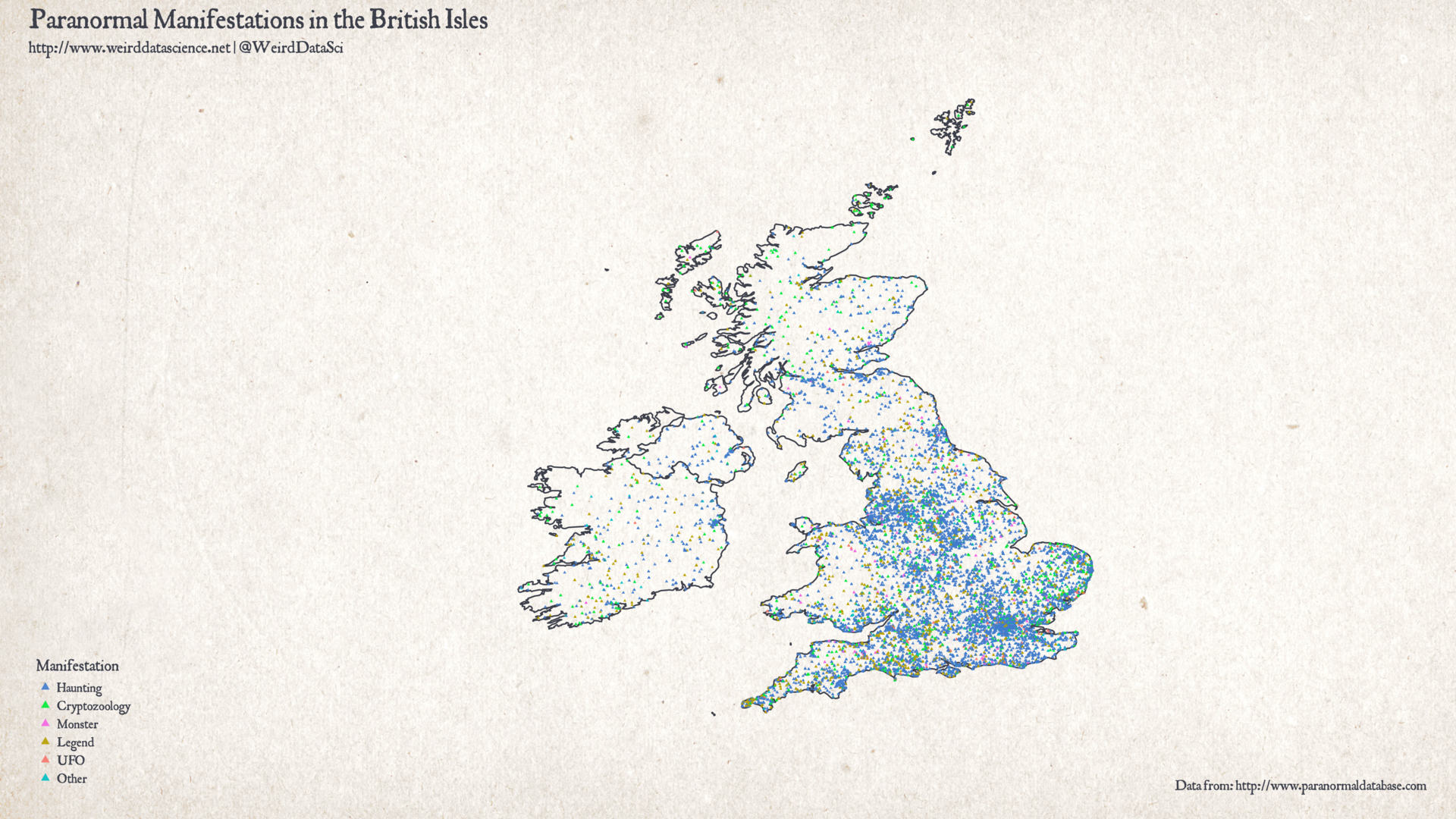
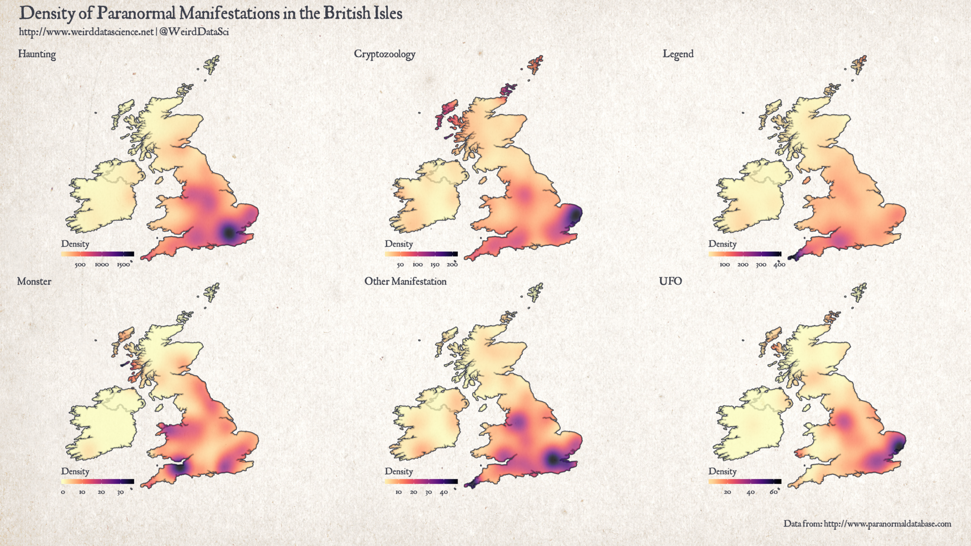
The maps are now updated with the Isle of Man. There’s a definite skew towards cryptozoology and legends, although there seem to be some hauntings down to the south-west.
Thank you for pointing out the oversight!
Excellent! Thank you.
BTW, I live in the Isle of Man
I had my suspicions!
However, your first png is still not showing IOM.
It has been updated, but may be cached in your browser — try a full refresh of the page.
Great – yes it’s there now. Thanks.
Excellent undertaking – this kind of visualisation is what I wanted to have as a tool for years and here you are. Is there also a way to connect the dots, by hovering over them with cursor, with any underlaying data, such as accounts files, book excerpts, newspaper clippings, footage, audio files, reports and so forth? Also, a time-beam placed below for the chronology of the data (progression over time)? And a selection tool for the various sub-phenomena?
Anyway, nice work!
Best regards,
Thei
Thank you!
If you look at the Global UFO Inquirer on a previous blog post: http://www.weirddatascience.net/blog/index.php/2018/02/22/unveiling-the-global-ufo-inquirer/ — direct link at http://laboratory.weirddatascience.net:3838/weirddatascience.net/global-ufo-inquirer — then that’s probably not dissimilar to what you’ve described there. Creating that sort of thing isn’t particularly hard once you’ve got the data.
The slight issue with the Paranormal Database data is that the location information is given as plain text. A good chunk of the work in producing this visualisation was plugging all of that into Google’s automatic location service and getting back latitudes and longitudes. That means that there’s almost certainly quite a few mislocated entries there. I don’t think it matters so much for the density heatmaps, but if I were to place each event on a map then there would be lots of inaccurate entries showing up. (The way to counter that would be to have a ‘report incorrect location’ link.)
Selection by type would be very easy once you had the basic map.
Timing is probably even more difficult. Again, the Paranormal Database lists times very informally: “unknown”, “some time in the 1800s”, “June 1937”, etc. That makes it difficult to create a time slider, as many events can’t be dated, and for others you would have to do a lot of work to turn it into computer-readable dates.
For the extra information, it’s very easy to link it to a popup like in the Global UFO Inquirer, if you have the data. You could start with the full entry on the Paranormal Database. I didn’t want to do it directly here, as that would effectively be duplicating the Paranormal Database, which felt rude. For linking to other sources, that would be a manual process. With over ten-thousand entries, that would be quite a task!
So, a lot of what you’re thinking is within the bounds of possibility. A location map with clickable events marked might happen in the future. For dates, and for other information sources, it would sadly require far more time than I have available!
I’m glad you like the maps, though. I’ll try to keep new and interesting things coming.
Is this still up to date? (amateur cryptid hunter and ghost hunter here)
The data for this was taken from the Paranormal Database, which is probably the best overall coverage of UK paranormal sightings and activity that exists — at least publicly. It was current at time of posting, and I don’t think the distributions are likely to have changed that much in the last few years!
I’ll say at this point that the owner of the Paranormal Database kindly agreed to share some data for analysis for future posts, and I feel bad that this post, and the previous one, was done by scraping the site directly. So, absolutely all credit to Darren Mann over at the Paranormal Database and thanks for being a great resource. At the same time, the Paranormal Database rightly points out that a lot of the sites listed there are private properties, so do take that into account when you’re plunging relentlessly into the darkness of our shared cultural psyche.
Good luck with the hunts! Happy to hear back anything you discover. I have a new series of blog posts, and another Halloween Lecture, in the process of being written up, as well as plans for the future, so hopefully Weird Data Science will become a little more active again in the near future.
I’ll be sure to write a few of my discoveries here before attempting to submit them to either the Paranormal Database or just adding em to the cryptid fandom wiki (or just making my own because fandom is absolutely terrible